Automatically Differentiable Weak Lensing Simulations for Full-Field Cosmological Inference
Denise Lanzieri


Cosmological N-Body Simulations
How do we simulate the Universe in a fast and differentiable way?
The Particle-Mesh scheme for N-body simulations
The idea: approximate gravitational forces by estimating densities on a grid.- The numerical scheme:
- From the particle positions estimate the density of particles on a mesh
- Apply a Fourier transform to obtain the over-density field $\delta_k$ in Fourier space.
- Compute gravitational forces $\to$ related to the density field via a transfer function ($\nabla \nabla^{-2}$)
- Interpolate back the force at every particle position
Fill the gap in the accuracy-speed space
-
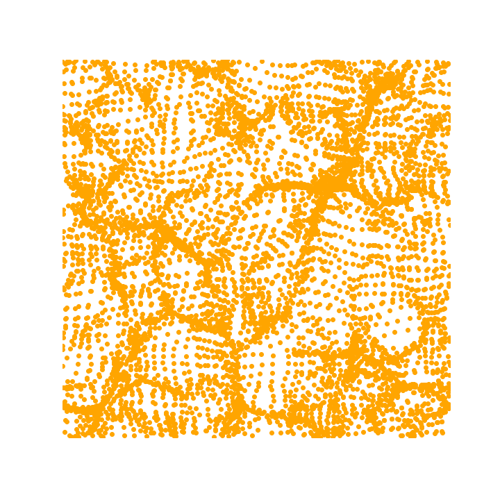
N-body PM simulation:
- Fast (we don't solve the full N-body problem)
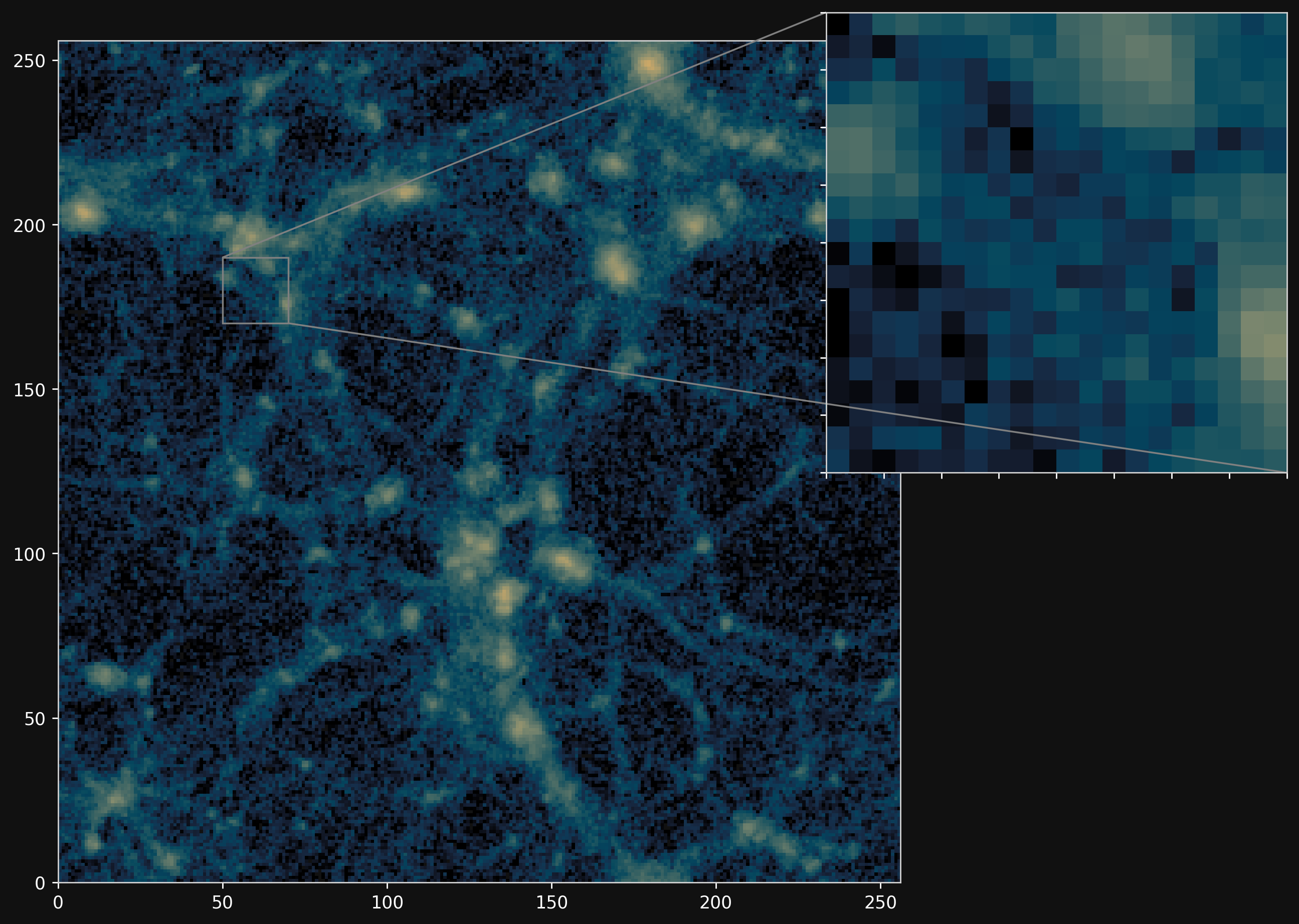
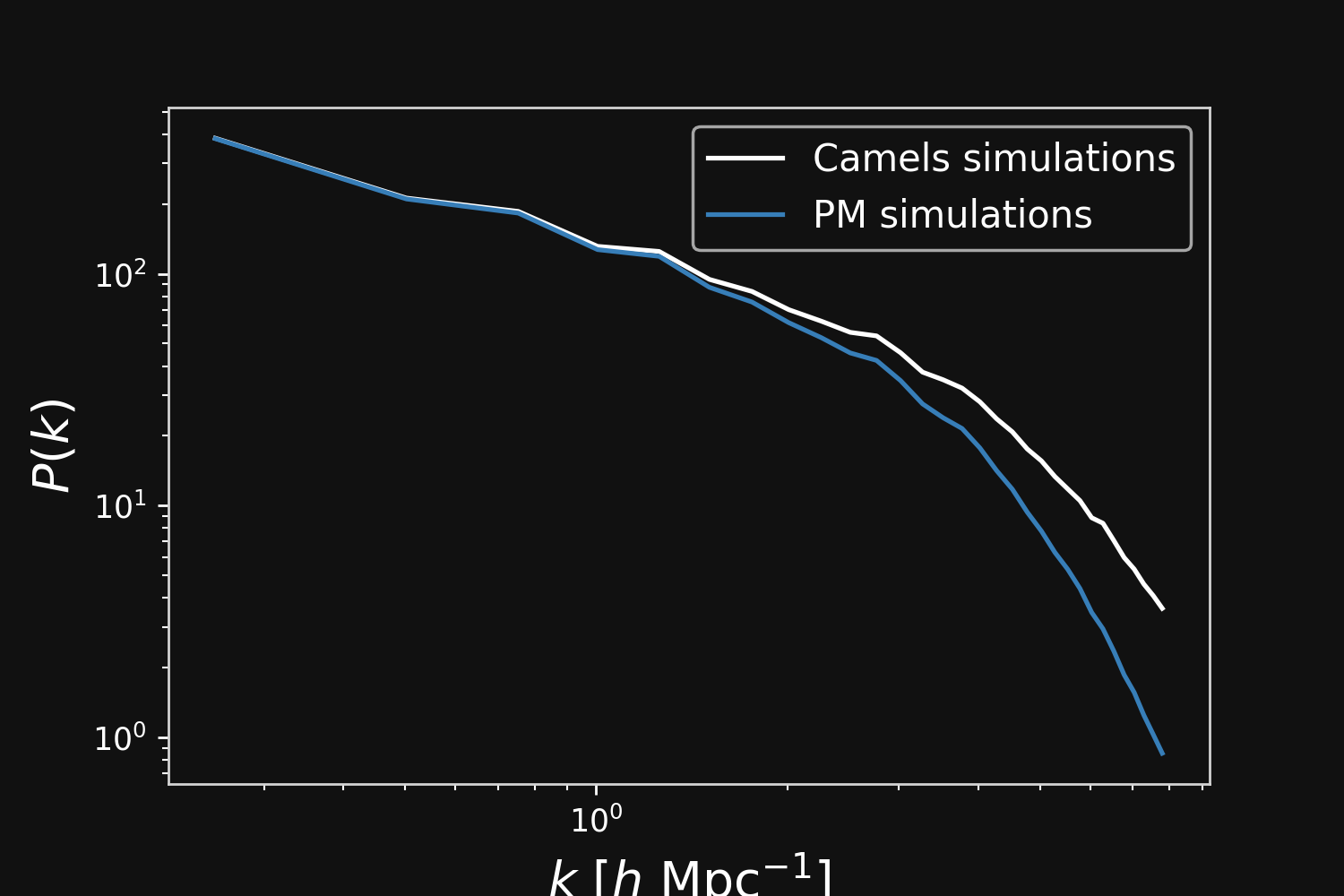
- Not able to resolve structures with scales smaller than the mesh resolution
- $\to$ Overdensity structures less sharp than full N-body counterparts
- $\to$ Lack power on small scales
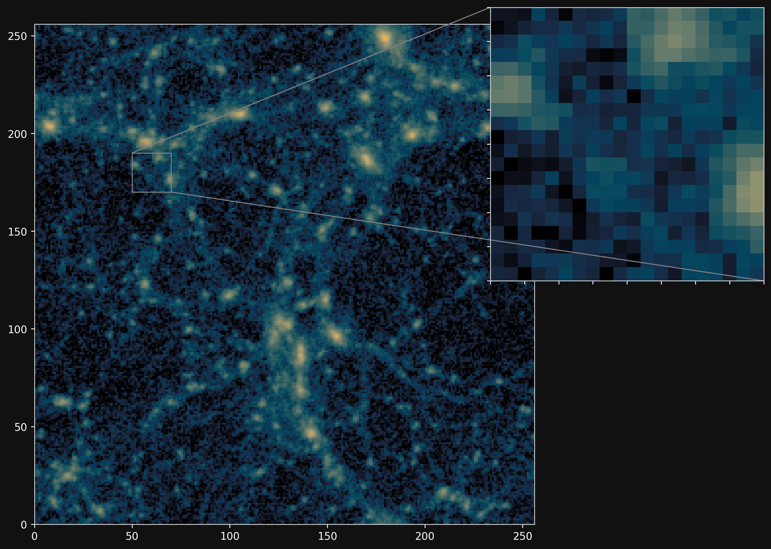
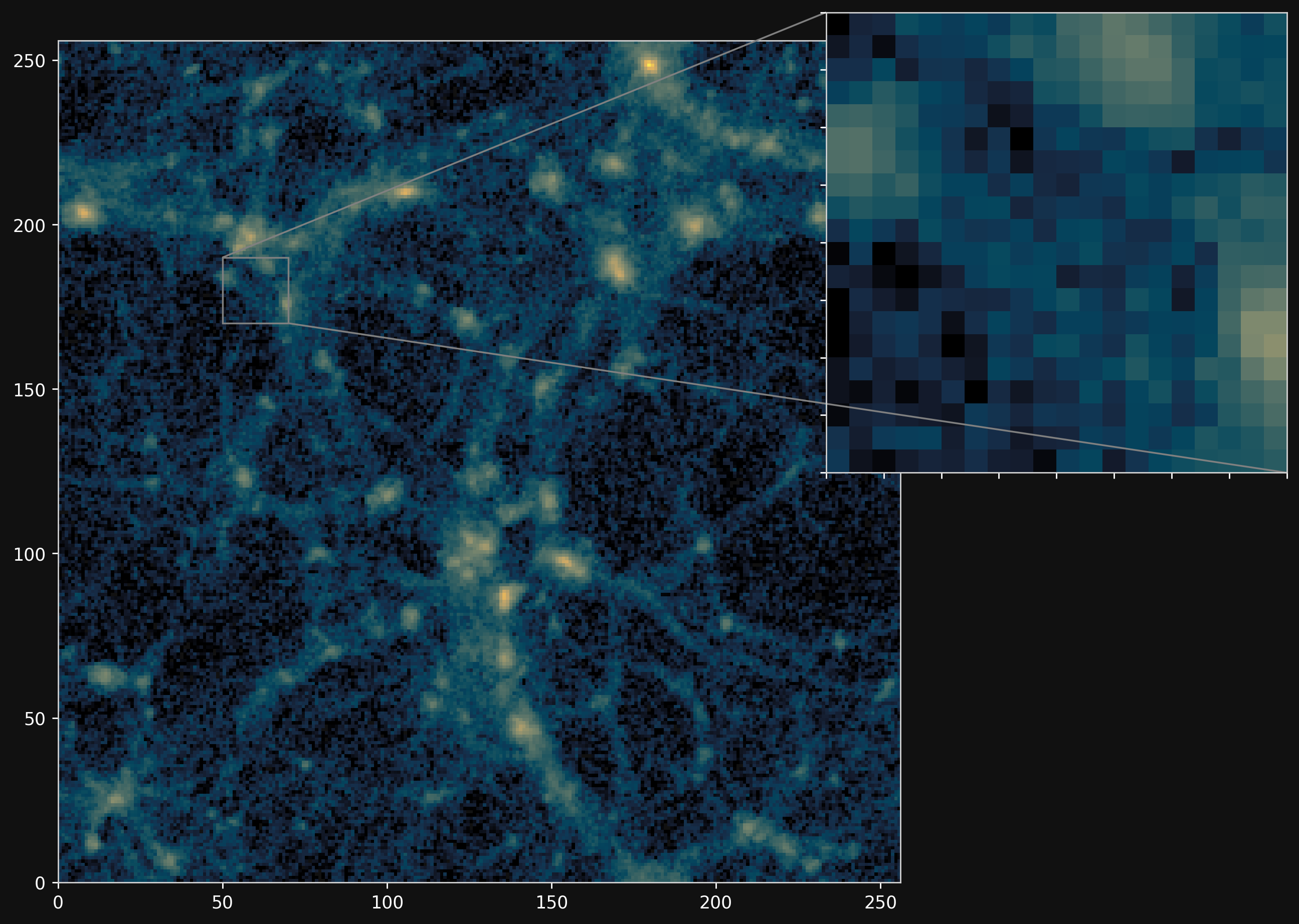
Camels simulations
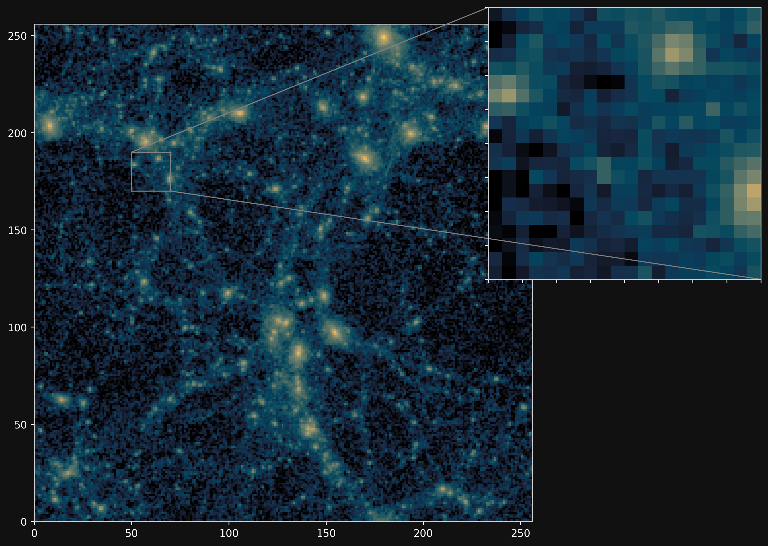
PM simulations
Hybrid Physical-Neural ODEs for Fast N-body Simulations
- Fast realization of complex processes
- $\Longrightarrow$ Take the effective physics description and combine it with a ML approach
- Cosmological simulations are based on physical processes
- $\Longrightarrow$ These impose symmetries and constraints
Augment the physical equations with a neural network
We compute the time integration from a system of ordinary differential equations (ODE) $$\left\{ \begin{array}{ll} \frac{d \color{#6699CC}{\mathbf{x}} }{d a} & = \frac{1}{a^3 E(a)} \color{#6699CC}{\mathbf{v}} \\ \frac{d \color{#6699CC}{\mathbf{v}}}{d a} & = \frac{1}{a^2 E(a)} F_\theta( \color{#6699CC}{\mathbf{x}} , a), \\ F_\theta( \color{#6699CC}{\mathbf{x}}, a) &= \frac{3 \Omega_m}{2} \nabla \left[ \color{#669900}{\phi_{PM}} (\color{#6699CC}{\mathbf{x}}) \right] \end{array} \right. $$
- $\mathbf{x}$ and $\mathbf{v}$ define the position and the velocity of the particles
- $\phi_{PM}$ is the gravitational potential in the mesh
$\to$ We can use this parametrisation to complement the physical ODE with neural networks.
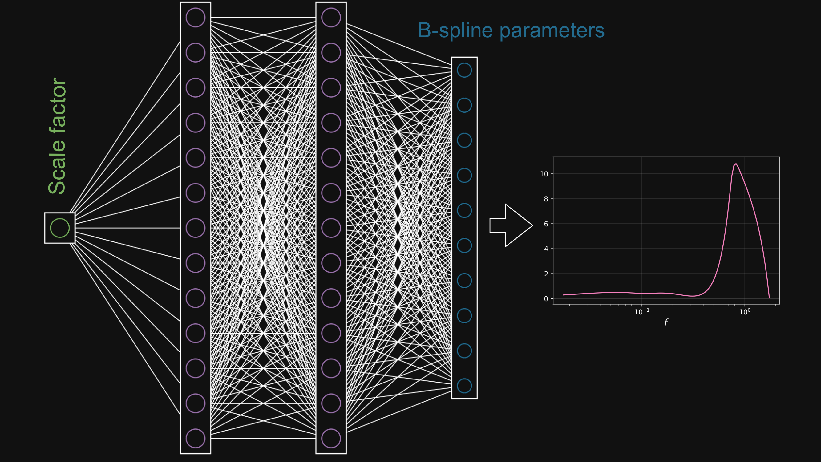
$$F_\theta(\mathbf{x}, a) = \frac{3 \Omega_m}{2} \nabla \left[ \phi_{PM} (\mathbf{x}) \ast \mathcal{F}^{-1} (1 + \color{#996699}{f_\theta(a,|\mathbf{k}|)}) \right] $$
Learn the Neural Filter
- $f_{\theta}(a)$ is defined as B-spline functions whose coefficients are the output of the Neural Network of parameters $\theta$.
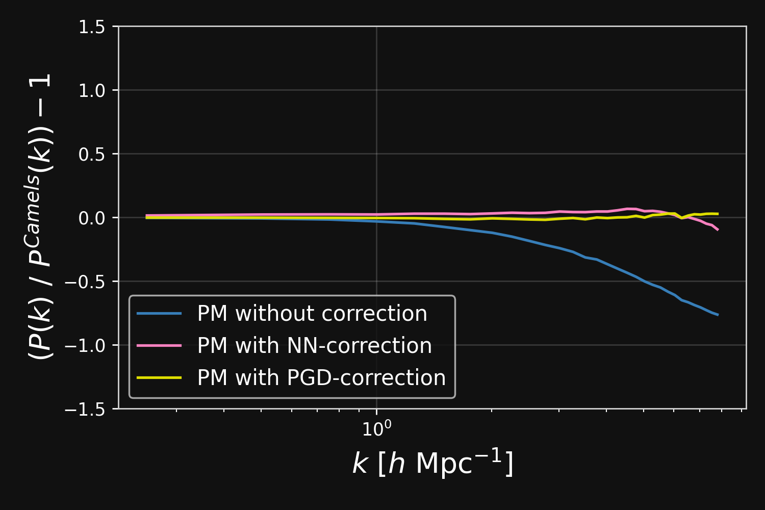
Train and validation loss
- We adopt a loss function penalizing both the particle positions and the overall matter power spectrum at different snapshot times
- We train and compare the model to the CAMELS simulations (Villaescusa-Navarro et al., 2021)
- We use a single N-body simulation of $25^3$ ($h^{-1}$ Mpc)$^3$ volume, $64^3$ dark matter particles at the fiducial cosmology of $\Omega_m = 0.3$ and $\sigma_8 = 0.8$
- Whole code implemented in the Python package Jax.
Backpropagation through the ODE solver
We are following the technique from Neural ODEs to backpropagate through an ODE solver (Neural Ordinary Differential Equations, Chen et al. 2018).To optimize $\textbf{L}$, we require gradients with respect to $\theta$:
- Determine how the gradient of the loss (the adjoint) depends on the hidden state $z$(t) at each instant: $$\color{#669900}{\textbf{a}}(t)=\frac{\partial \color{#6699CC}{L}}{\partial \color{#996699}{\textbf{z}}(t)}$$
- Compute the adjoint dynamics by solving a another ODE: $$ \frac{d\color{#669900}{\textbf{a}}(t)}{dt}=\color{#669900}{\textbf{a}}(t)^{T}\frac{\partial f(\color{#996699}{\textbf{z}}(t),t,\color{#ecad60}{\theta})}{\partial \color{#996699}{\textbf{z}}} $$
- Compute the gradients with respect to the parameters $\theta$ evaluating a third integral: $$ \frac{d\color{#6699CC}{L}}{d\color{#ecad60}{\theta}}=\int_{t_1}^{t_0}\color{#669900}{\textbf{a}}(t)^T \frac{\partial f (\color{#996699}{\textbf{z}}(t),t,\theta)}{\partial \color{#ecad60}{\theta}}dt $$
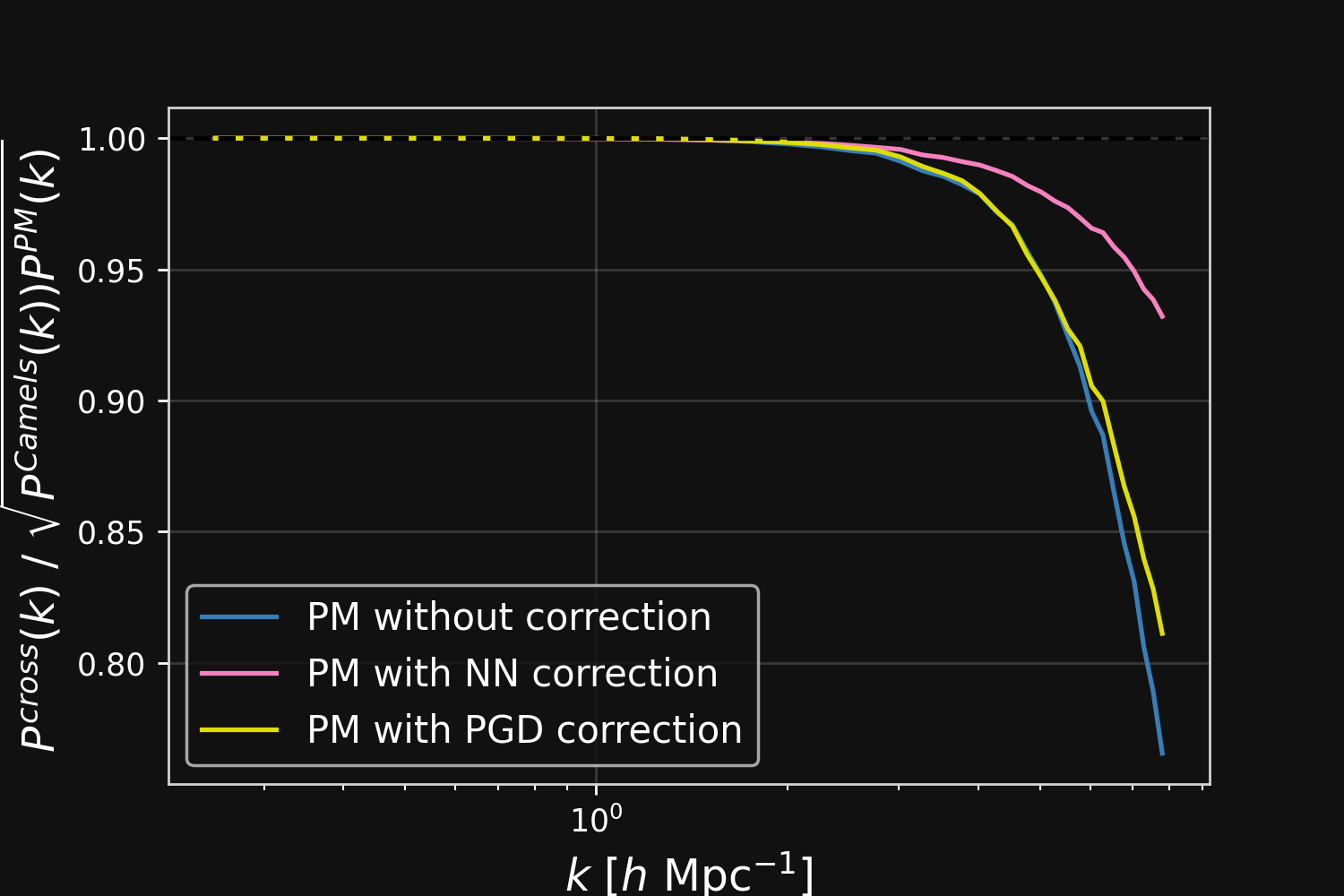
Hybrid Physical-Neural ODE
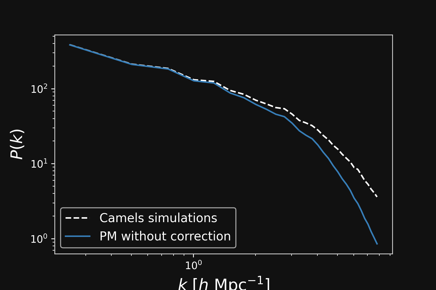
Without neural correction
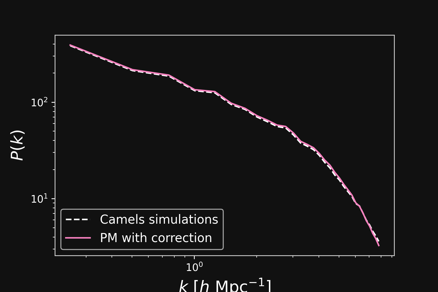
With neural correction
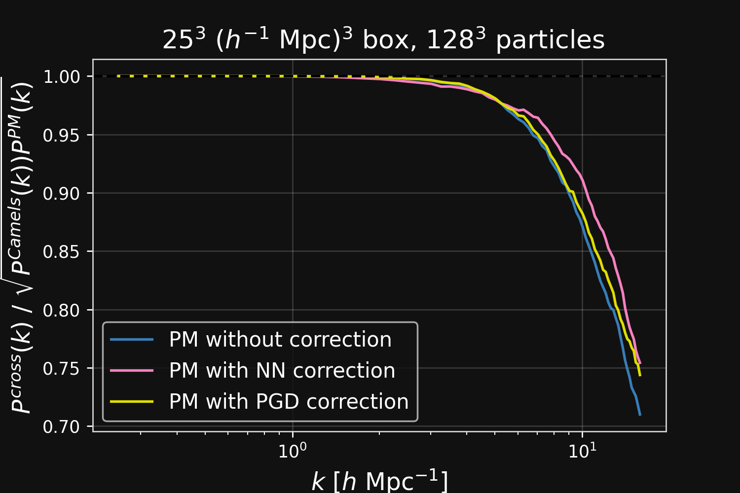
Results
Results: Robustness to changes in resolution and cosmological parameters
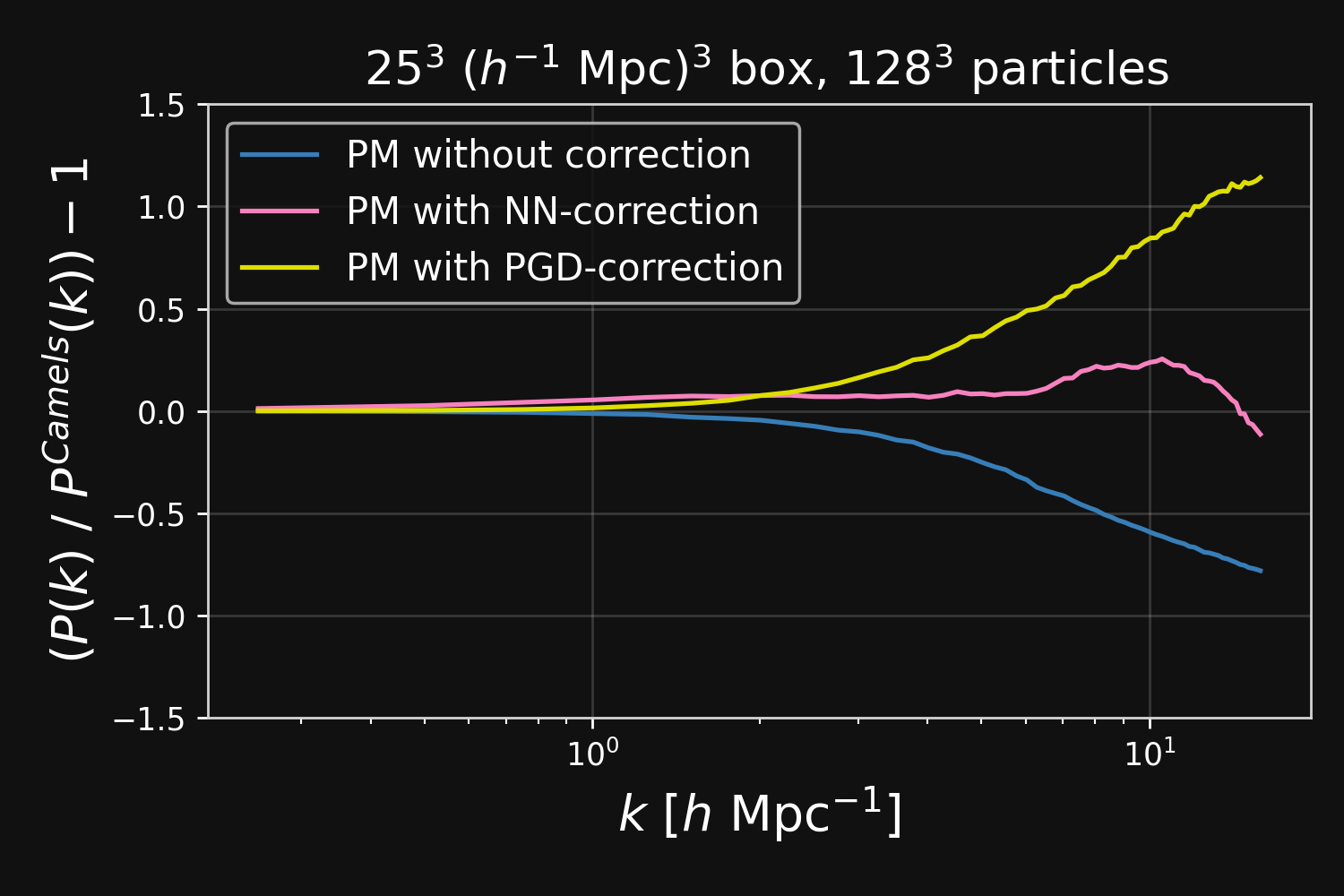
Higher resolution
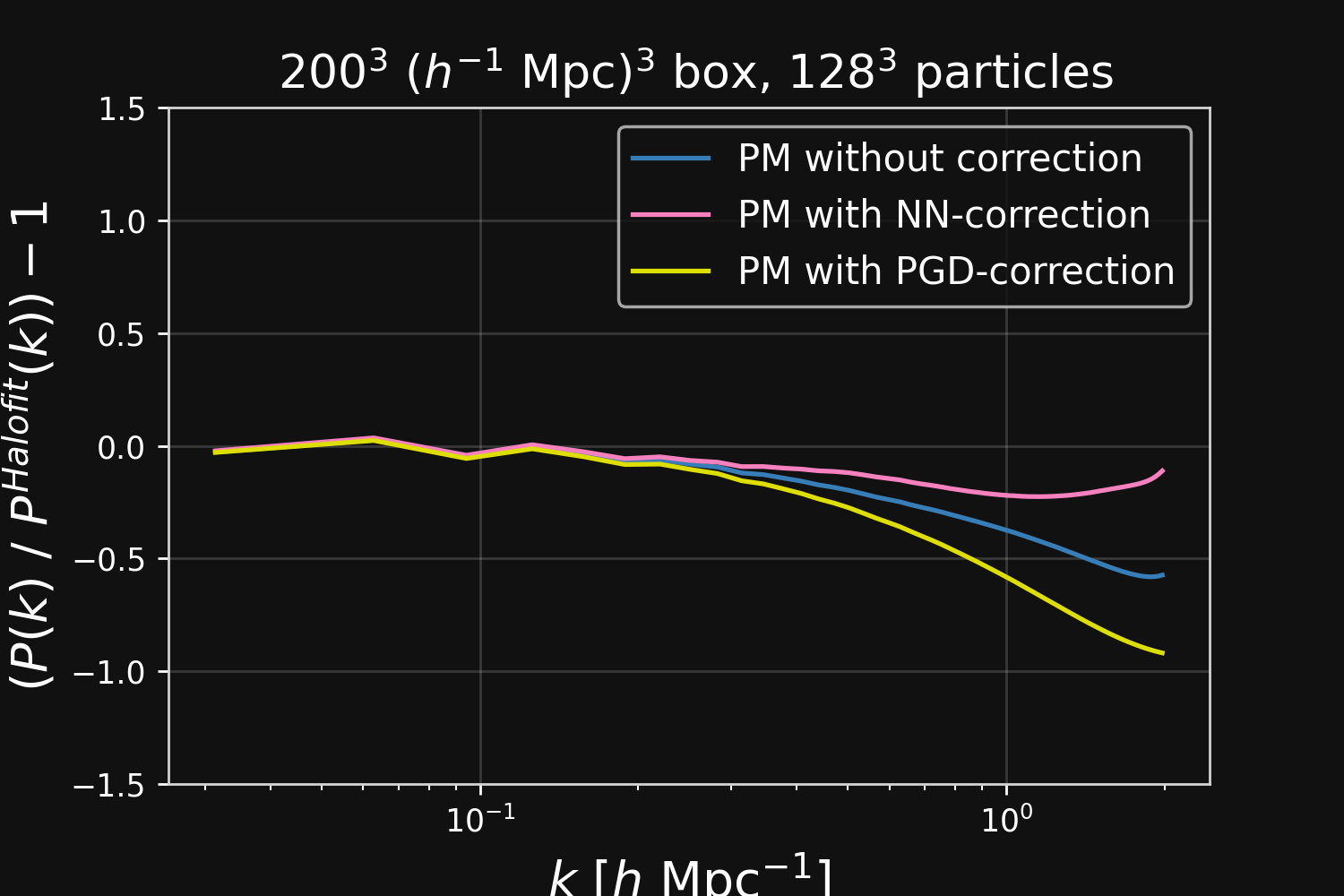
Lower resolution
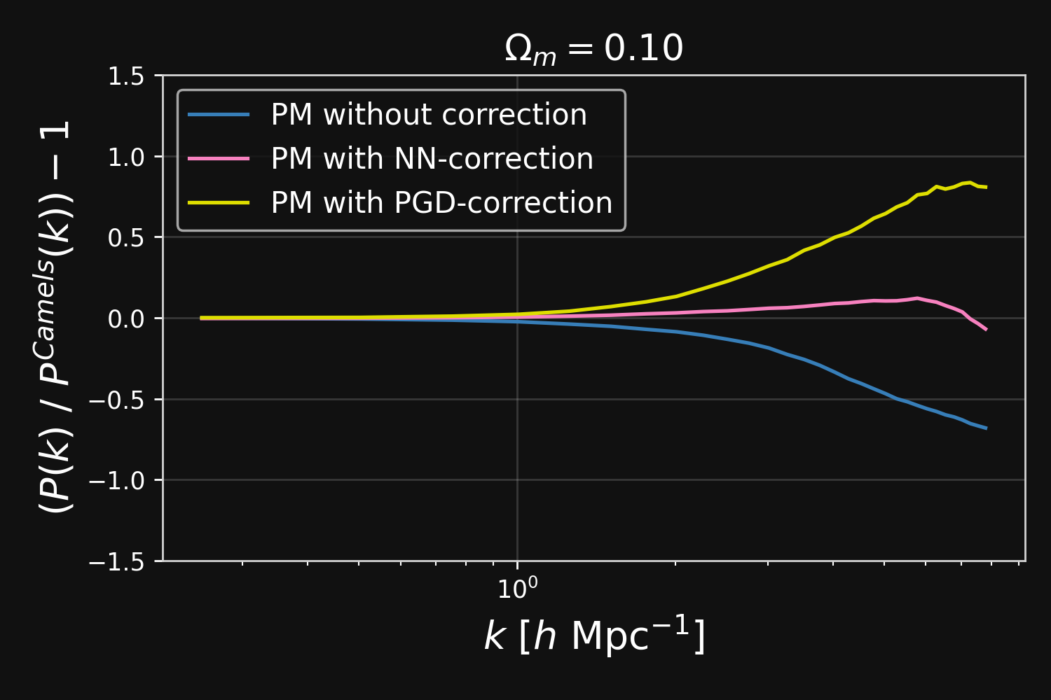
Different Cosmology
Example use-case: Forecasting the power of Higher Order Weak Lensing Statistics with automatically differentiable simulations
Work in collaboration with:
F. Lanusse, C. Modi, B. Horowitz, J. Harnois-Déraps, J.L. Starck,
The LSST Dark Energy Science Collaboration (LSST DESC)
$\Longrightarrow$ Compare the constraining power of weak lensing statistics and investigate the degeneracy in high dimensional cosmological parameter space.
Introducing FlowPM: Particle-Mesh Simulations in TensorFlow


										import tensorflow as tf
										import flowpm
										# Defines integration steps
										stages = np.linspace(0.1, 1.0, 10, endpoint=True)

										initial_conds = flowpm.linear_field(32,       # size of the cube
																			100,       # Physical size
																			ipklin,    # Initial powerspectrum
																			batch_size=16)

										# Sample particles and displace them by LPT
										state = flowpm.lpt_init(initial_conds, a0=0.1)

										# Evolve particles down to z=0
										final_state = flowpm.nbody(state, stages, 32)

										# Retrieve final density field
										final_field = flowpm.cic_paint(tf.zeros_like(initial_conditions),
																		final_state[0])
Differentiable Lensing Lightcone: TensorFlow-based weak gravitational lensing package
-
We extend the FlowPM approach:
- Computing the time integration starting from a system of ODE.
- Tune the accuracy-speed by defining a tolerance of the ODE Solver
- Reduced memory usage: no need to store intermediate steps for backpropagation.
- Integrating the Hybrid Physical-Neural parameterisation to compensate for the small-scale approximations
- Implementing ray-tracing and simulating lensing lightcones in the Tensorflow framework
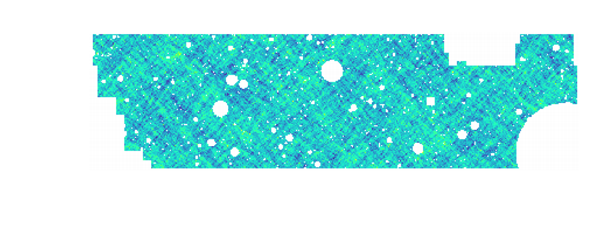
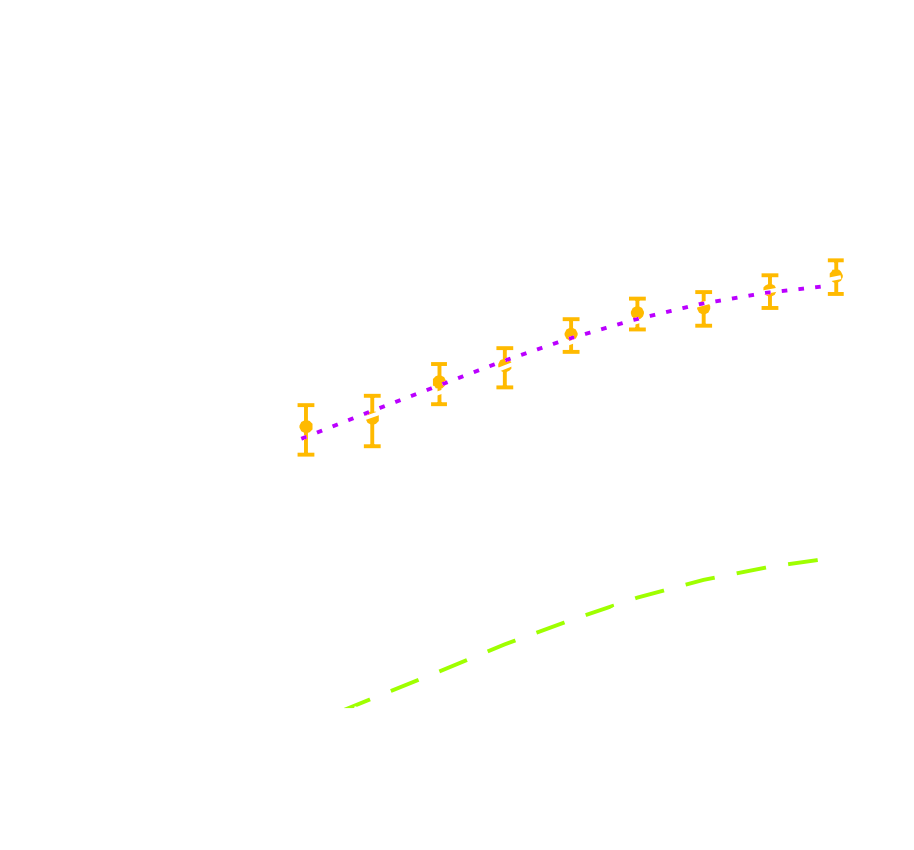
Validating simulations: Lensing $C_{\ell}$
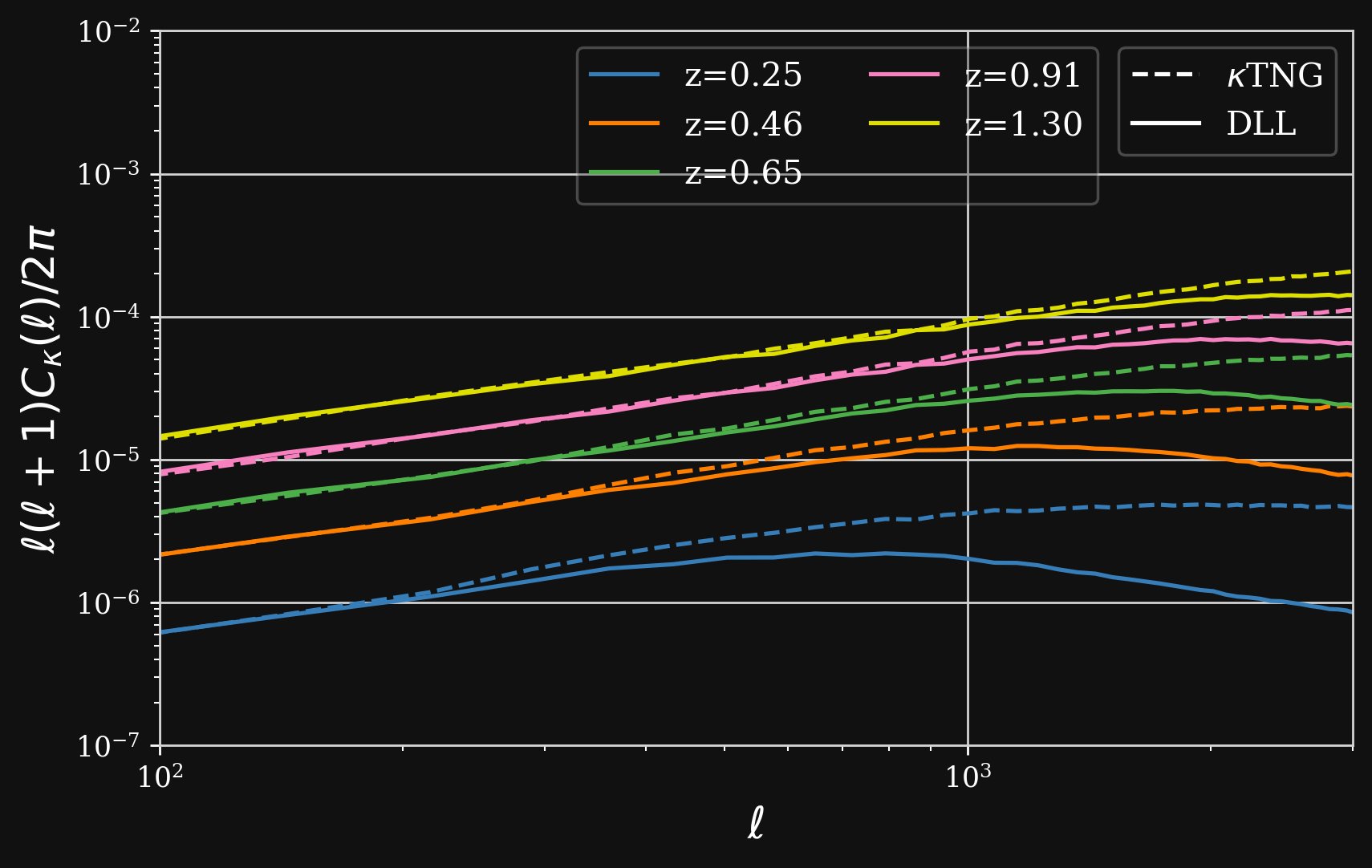
- Predictions from DLL simulations ($128^3$ particles, box size of 205 Mpc/h ) against $\kappa$TNG ($2500^3$ particles, box size of 205 Mpc/h )
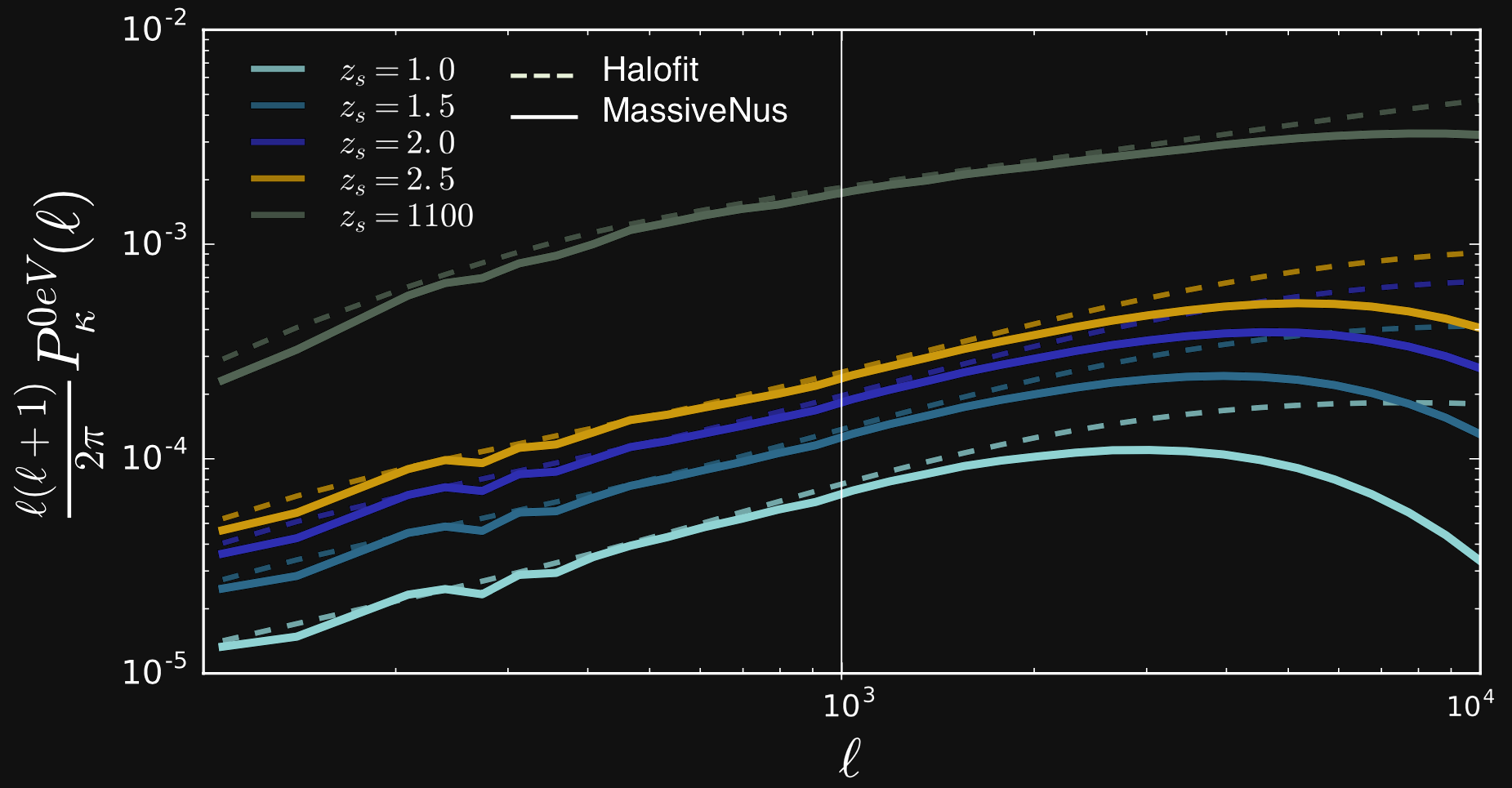
- Predictions from MassiveNus simulations ($1024^3$ particles, box size of 512 Mpc/h) against Halofit.
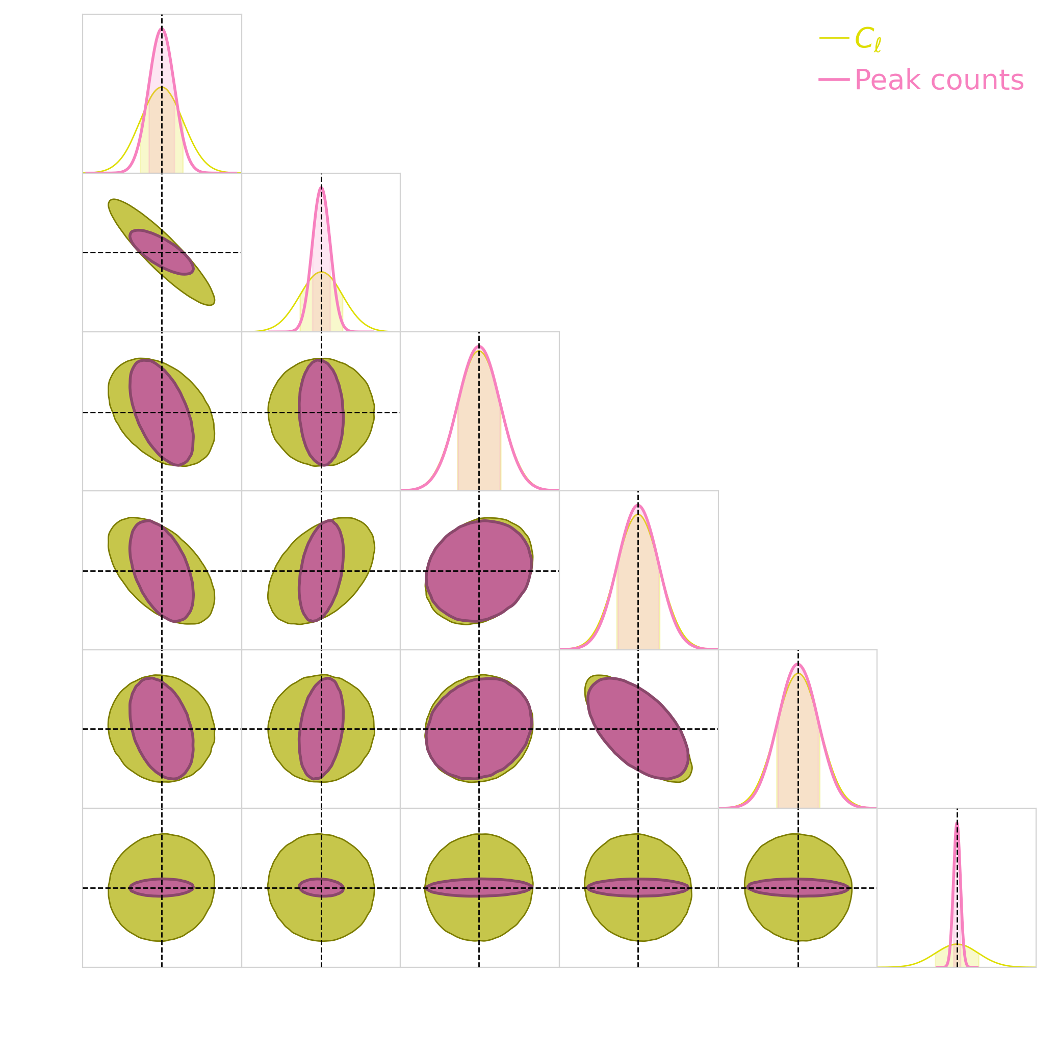
Compare the information content
(Results presented on behalf of LSST DESC)
- Use Fisher matrix to estimate the information content extracted with a given statistic
- Derivative of summary statistics respect to the cosmological parameters.
- Fisher matrices are notoriously unstable
$\Longrightarrow$ they rely on evaluating gradients by finite differences. - They do not scale well to large number of parameters.
Compare the information content
- Use Fisher matrix to investigate the degeneracy between the cosmological parameters in high dimensional space and when systematics are included in the analysis.
Conclusion
- Powerful ways to simulate fast cosmological simulations
- Data driven way of complementing a physical models
- correction scheme to compensate for the small-scales approximations preserving translation and rotation symmetries
- Automatically differentiable physical models for fast inference
- Likelihood-free inference approach
- Inference of the full posterior distribution by using the Hamiltonian Monte Carlo (HMC) method
GitHub repo:
DifferentiableUniverseInitiative/jaxpm-paper
DifferentiableUniverseInitiative/flowpm
LSSTDESC/DifferentiableHOS
Thank you !
APPENDIX
the $\Lambda$CDM view of the Universe


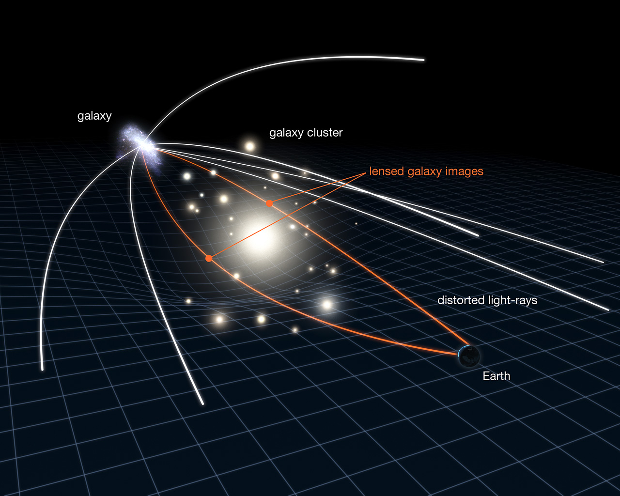
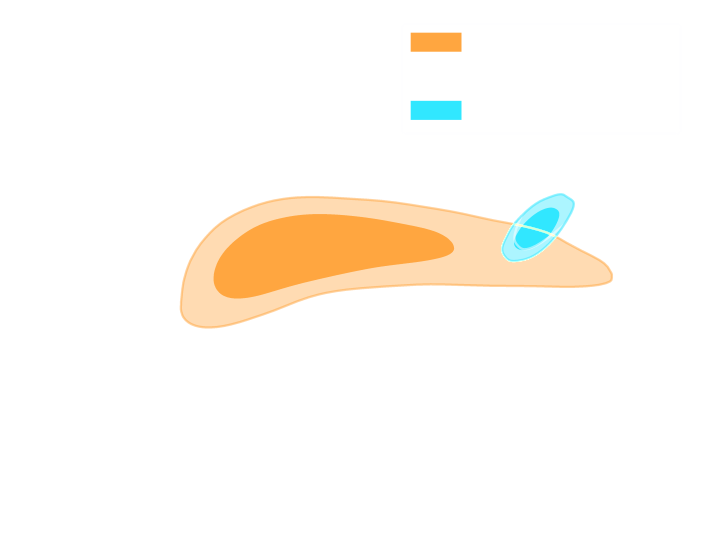
Weak Gravitational lensing
The limits of traditional cosmological inference
- Measure the ellipticity $\epsilon = \epsilon_i + \gamma$ of all galaxies
$\Longrightarrow$ Noisy tracer of the weak lensing shear $\gamma$ - Compute summary statistics based on 2pt functions,
e.g. the power spectrum - Run an MCMC to recover a posterior on model parameters, using an analytic likelihood $$ p(\theta | x ) \propto \underbrace{p(x | \theta)}_{\mathrm{likelihood}} \ \underbrace{p(\theta)}_{\mathrm{prior}}$$
- Implicit Inference: Treat the simulator as a black-box with only the ability to sample from the joint distribution
$$(x, \theta) \sim p(x, \theta)$$
a.k.a.
- Simulation-Based Inference (SBI)
- Likelihood-free inference (LFI)
- Approximate Bayesian Computation (ABC)
- Explicit Inference: Treat the simulator as a probabilistic model and perform inference over the joint posterior
$$p(\theta, z | x) \propto p(x | z, \theta) p(z | \theta) p(\theta) $$
a.k.a.
- Bayesian Hierarchical Modeling (BHM)
Mesh FlowPM: distributed, GPU-accelerated, and automatically differentiable simulations
- We developed a Mesh TensorFlow implementation that can scale on GPU clusters (horovod+NCCL).
- For a $2048^3$ simulation:
- Distributed on 256 NVIDIA V100 GPUs
- Runtime: 3 mins
- Don't hesitate to reach out if you have a use case for model parallelism!
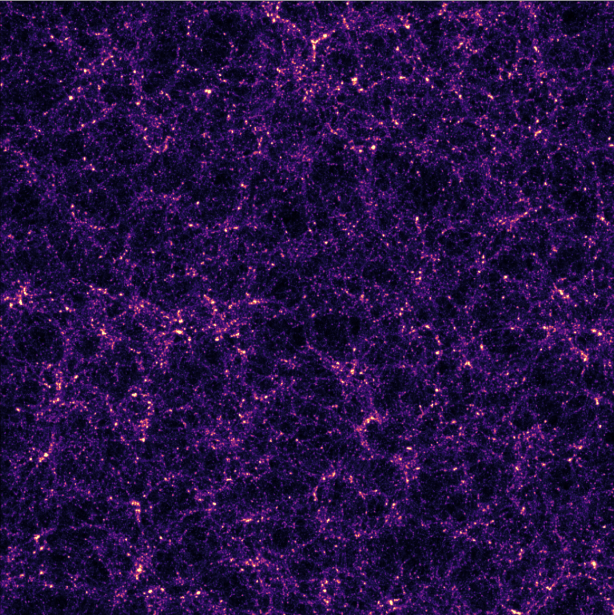
![]()
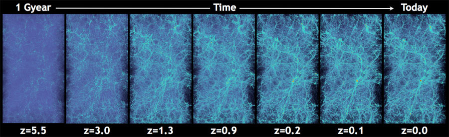
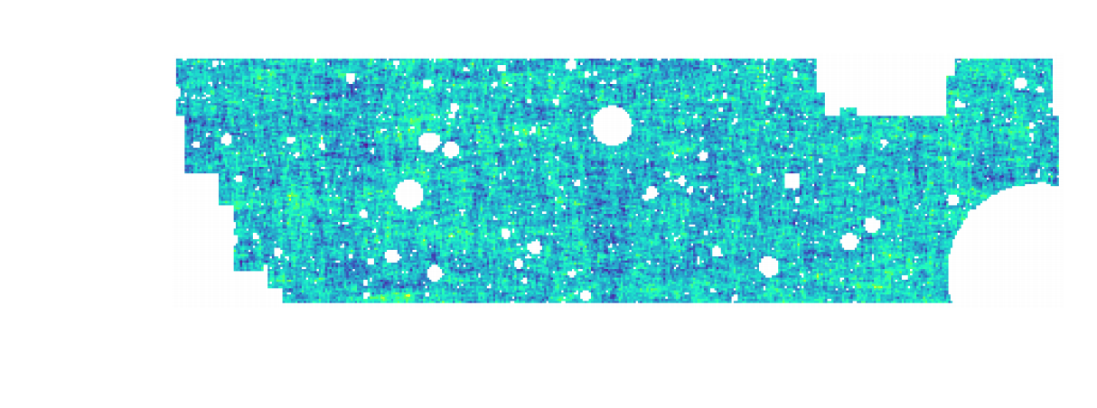
Projections of final density field
Results: Robustness to changes in resolution and cosmological parameters
Higher resolution
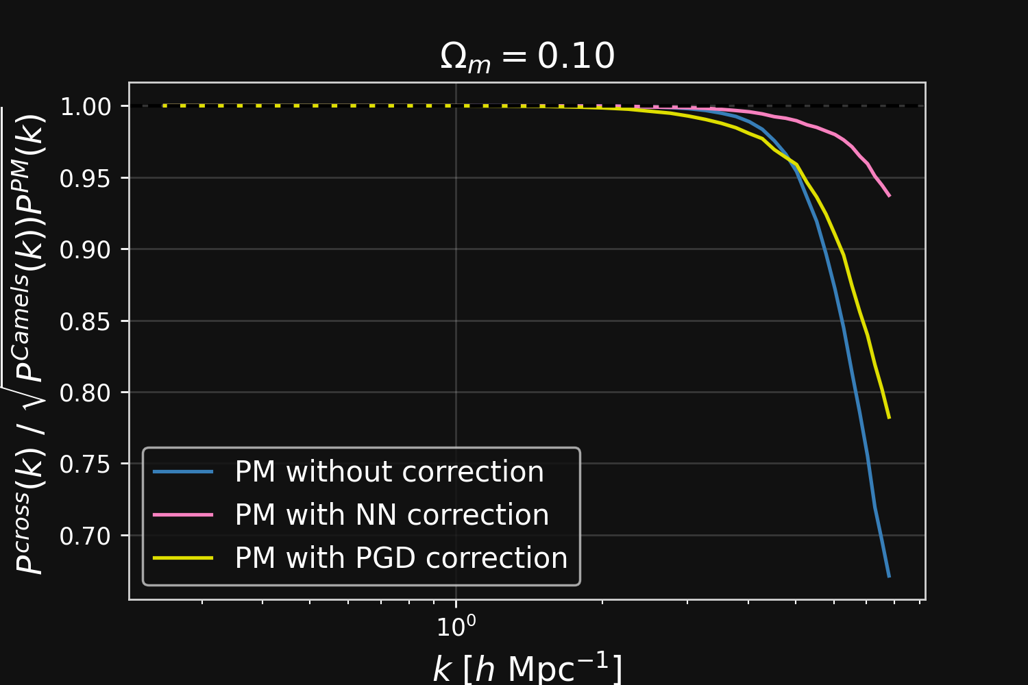
Different Cosmology!
Proof of Concept
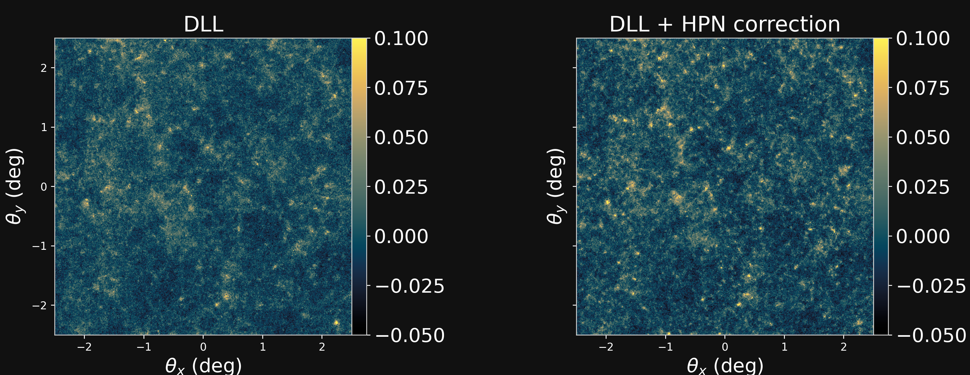
Validating simulations: HPN validation
Predictions of DLL simulations before and after using the Hybrid Physical-Neural against $\kappa$TNG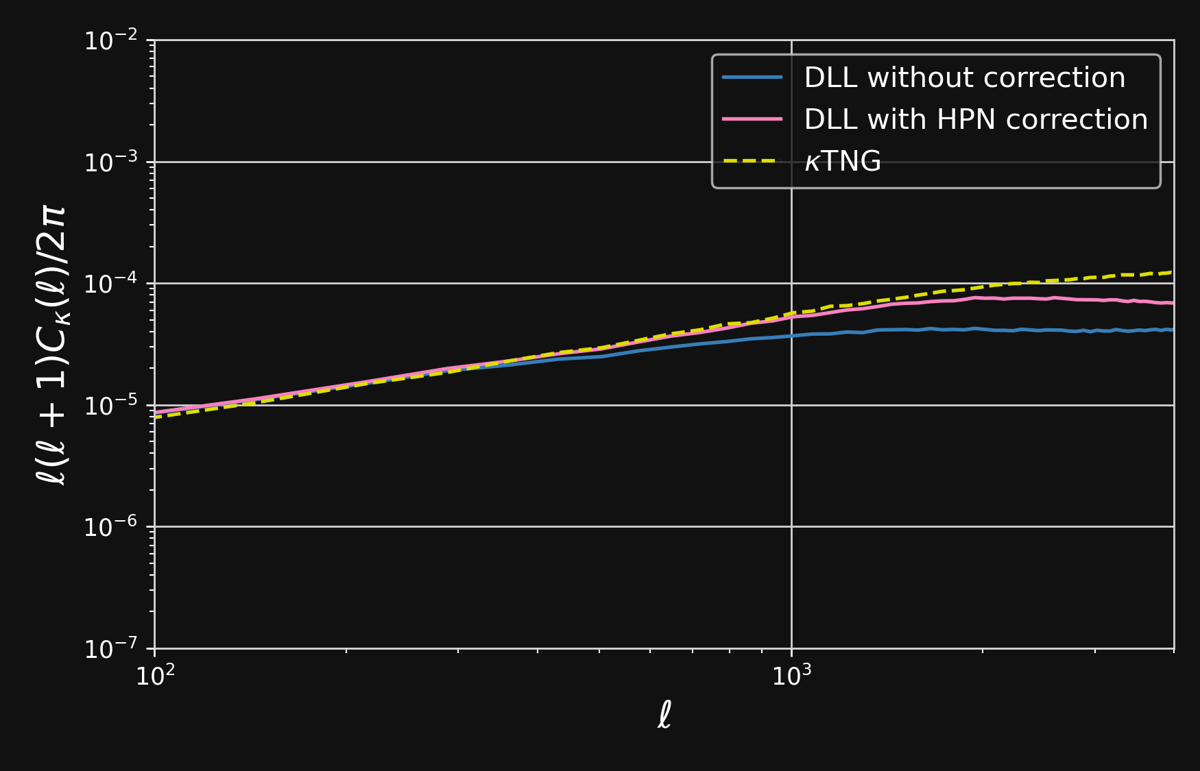
$C_{\ell}$
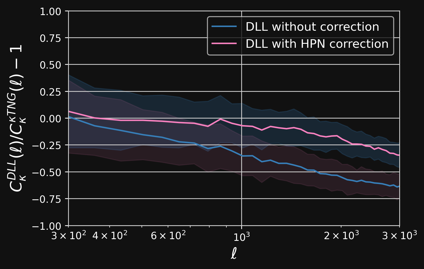
Fractional $C_{\ell}$
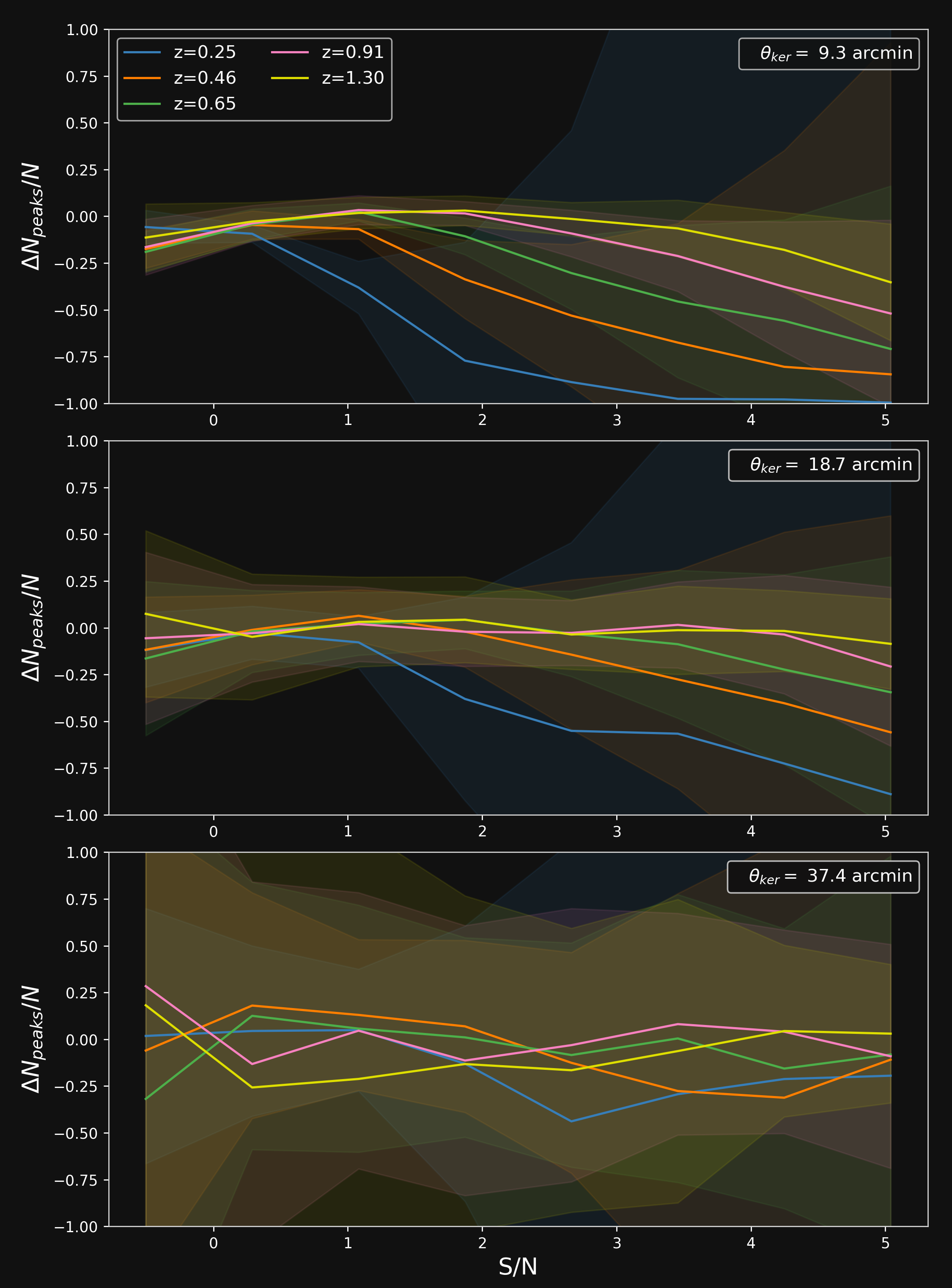
Validating simulations: Peak counts
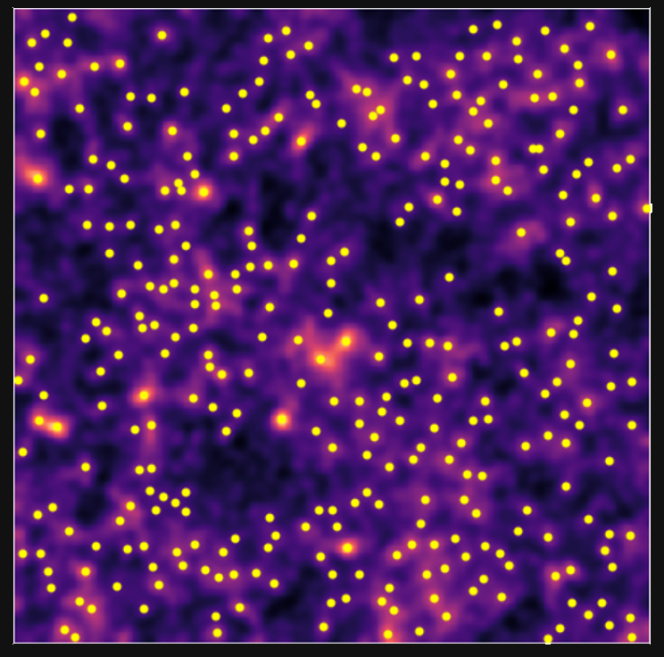
Validating simulations: Peak counts
Validating simulations: Peak counts
- Fractional number of peaks of DLL simulations and $\kappa$TNG simulations for different sources redshift.