Forecasting the power of Higher Order Weak Lensing Statistics with automatically differentiable simulations
Denise Lanzieri


slides at github.com/dlanzieri/talks/LSST_talk
the $\Lambda$CDM view of the Universe


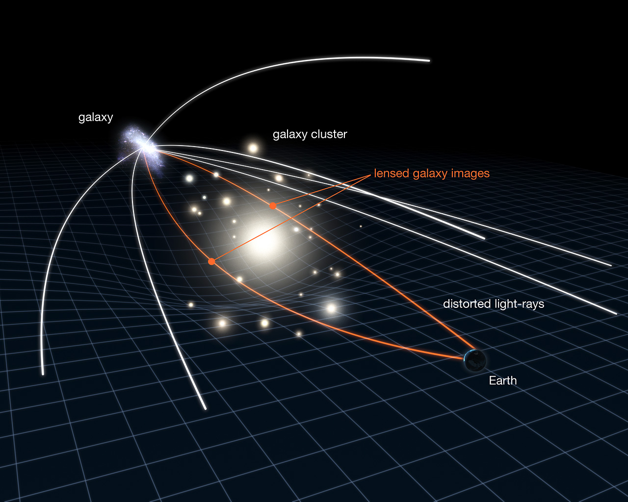
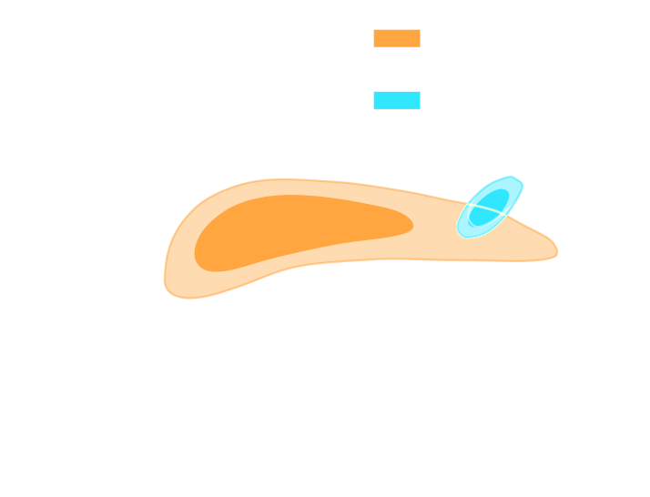
Weak Gravitational lensing
2 Point Statistics: A Suboptimal Measure
How do we make the most of the available data?
HSC cosmic shear power spectrum
HSC Y1 constraints on $(S_8, \Omega_m)$
(Hikage,..., Lanusse, et al. 2018)
- Shear $\gamma$
- Data reduction
- Power spectrum
Main limitation: The lensing convergence field is inherently and significantly non-Gaussian
The two-point statistics do not fully capture the non-Gaussian information encoded in the peaks of the matter distribution
$\Longrightarrow$ We are dismissing most of the information!
How to maximize the information gain?
Cosmological constraints from the combination of different summary statistics

(Ajani, et al. 2020)
- Approaches based on measuring high-order correlations to access the non-Gaussian information
e.g. the Peaks count
- Investigate the constraining power of various map-based higher order weak lensing statistics
- How can we do that in a fast and accurate way?
$\Longrightarrow$ Fisher Information
Fisher Matrix
\[\begin{equation}
F_{\alpha, \beta} =\sum_{i,j} \frac{d\mu_i}{d\theta_{\alpha}}
C_{i,j}^{-1} \frac{d\mu_j}{d\theta_{\beta}}
\end{equation} \]
- Use Fisher matrix to estimate the information content extracted with a given statistic
- Derivative of summary statistics respect to the cosmological parameters.
e.g. the $\Omega_c$, $\sigma_8$ - Estimate derivative with final differences
Numerical Differentiation
\[\begin{equation}
\left.\frac{df(x)}{dx}\right|_{x_1} \approx \frac{f(x_1+h)-f(x_1)}{h}
\end{equation} \]

-
Flaws :
- It’s numerically very unstable
- It’s very expensive in term of simulation time
- Computes an approximation
Different approach :
Automatic Differentiation
Automatic Differentiation
Automatic Differentiation and Gradients in TensorFlow
- TensorFlow compute automatically derivatives of arbitrary order by applying the chain rule repeatedly to elementary arithmetic operations
- To differentiate automatically, TensorFlow remember what operations happen in what order during the forward pass and traverses this list of operations in reverse order to compute gradients.
-
Advantages :
- Derivative as functions
- No numerical approximation
- High speed
Chain rule :
\[\begin{equation} \frac{dw}{du}=\frac{dw}{dv}\frac{dv}{du} \end{equation} \]
Cosmological N-Body Simulations
How do we simulate the Universe in a fast and differentiable way?
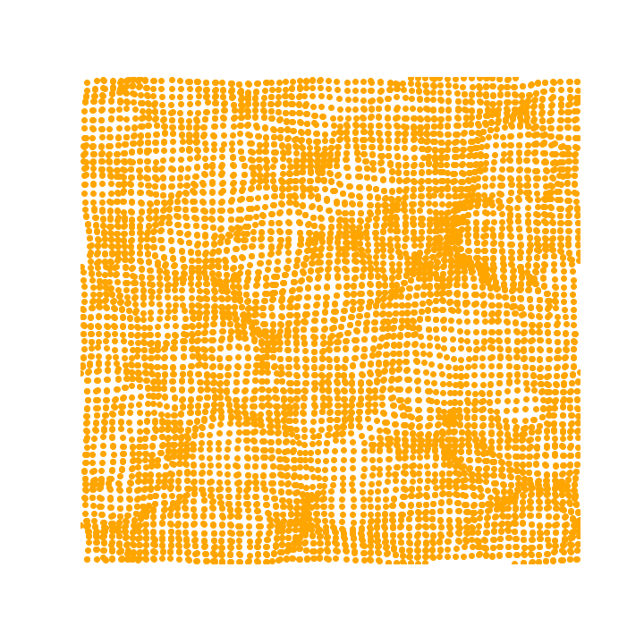
The Particle-Mesh scheme for N-body simulations
The idea: approximate gravitational forces by estimating densities on a grid.- The numerical scheme:
- Estimate the density of particles on a mesh
$\Longrightarrow$ compute gravitational forces by FFT - Interpolate forces at particle positions
- Update particle velocity and positions, and iterate
- Estimate the density of particles on a mesh
- Fast and simple, at the cost of approximating short range interactions.
$\Longrightarrow$ Only a series of FFTs and interpolations.
Introducing FlowPM: Particle-Mesh Simulations in TensorFlow

											import tensorflow as tf
											import flowpm
											# Defines integration steps
											stages = np.linspace(0.1, 1.0, 10, endpoint=True)

											initial_conds = flowpm.linear_field(32,        # size of the cube
											100,       # Physical size
											ipklin,    # Initial powerspectrum
											batch_size=16)

											# Sample particles and displace them by LPT
											state = flowpm.lpt_init(initial_conds, a0=0.1)

											# Evolve particles down to z=0
											final_state = flowpm.nbody(state, stages, 32)

											# Retrieve final density field
											final_field = flowpm.cic_paint(tf.zeros_like(initial_conditions),
											final_state[0])

											with tf.Session() as sess:
											sim = sess.run(final_field)
- Seamless interfacing with deep learning components

Mocking the weak lensing universe:
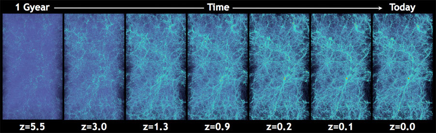
- We can map the distribution of all matter over cosmic time.
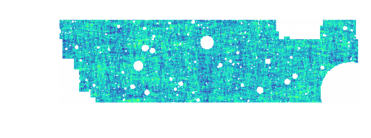
- Convergence maps
$\Longrightarrow$ weighted projection of the 3D cosmological mass density along the line-of-sight. - Access the signal in the convergence maps using a given statistic, e.g. Convergence power spectrum
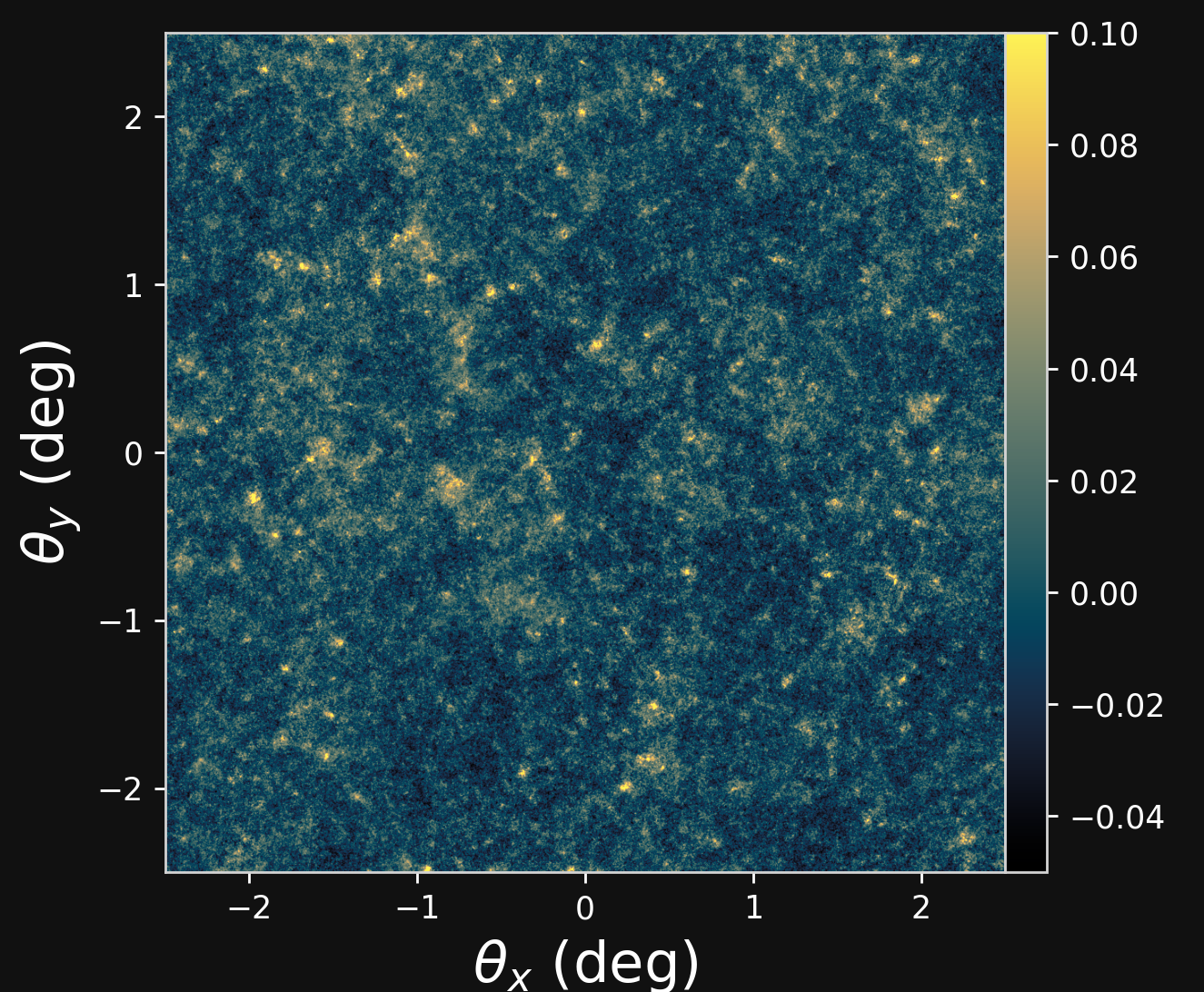
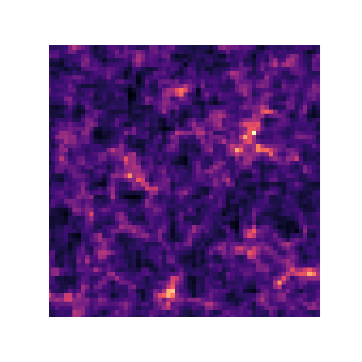
Convergence map at z=1.0, based on a 3D simulation of side length 256 Mpc/h and $256^3$ particles. (Böhm, et al. 2020)
Mocking the weak lensing universe: The Born Approximation
- Numerical simulation of WL features rely on ray-tracing through the output of N-body simulations
- Knowledge of the Gravitational potential and accurate solvers for light ray trajectories is computationally expensive
- Born approximation , only requiring knowledge of the density field, can be implemented more efficiently and at a lower computational cost
\[\begin{equation} \kappa_{born}(\boldsymbol{\theta},\chi_s)= \frac{3H_0^2 \Omega_m}{2c^2} \int_0^{\chi_s} d\chi \frac{\chi}{a(\chi)} W(\chi,\chi_s) \delta(\chi \boldsymbol{\theta},\chi). \end{equation} \]
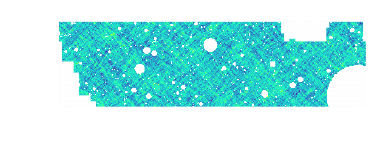
Raytracing Validation
We simulate lensing lightcones implementing gravitational lensing ray-tracing in FlowPM framework

Proof of Concept
- Convergence map at z=1.0, based on a 3D simulation of $64^3$ particles for side. The 2D lensing map has an angular extent of $5^{\circ}.$
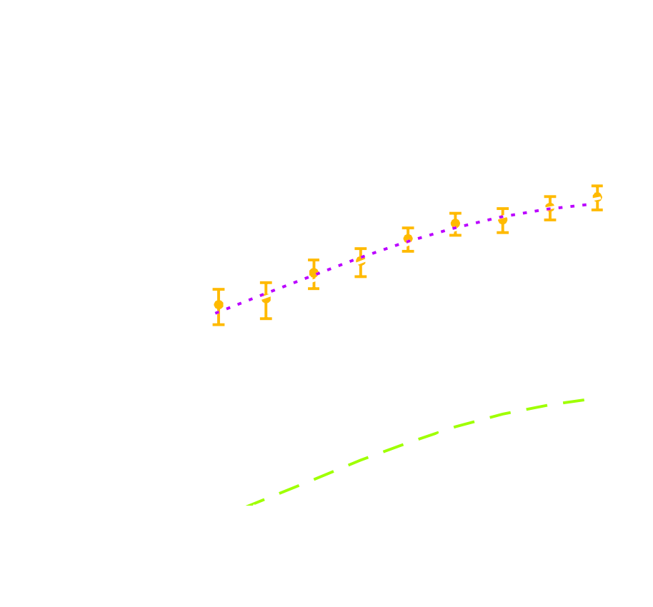
- Angular Power Spectrum $C_\ell$
- The Jacobian: \[\begin{equation} \frac{dC_l}{d\Omega_c}, \frac{dC_l}{d\sigma_8} \end{equation} \] \[\begin{equation} F_{\alpha, \beta} =\sum_{i,j} \frac{d\mu_i}{d\theta_{\alpha}} C_{i,j}^{-1} \frac{d\mu_j}{d\theta_{\beta}} \end{equation} \]
-
Constraints on cosmological parameter $\Omega_c$ and $\sigma_8$:


Status and Next steps
- Distributed version of FlowPM on several GPUs to generate large-scale mass-maps
- Peak counts statistic implement in TensorFlow framework
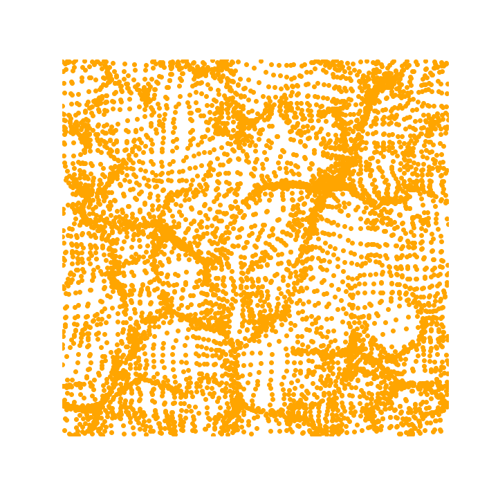
- Weak lensing peaks trace regions where the value of the convergence field is high $\Longrightarrow$ they are associated to massive Structures.
- We compute peaks as local maxima of the signal-to-noise field
- Compute summary statistic higher than second order to extract non-Gaussian cosmological information and infer cosmological parameters
Conclusion
Conclusion
What can be gained by simulating the Universe in a fast and differentiable way?
- Differentiable physical models for fast inference
- Forecasts on differentiable higher-order statistics, including peak counts, etc.
- Investigate the constraining power of various map-based higher order weak lensing statistics
Conclusion
Everyone is most welcome to join! How to get in touch:
- Confluence page
- Slack channel #desc-wl-massmap, and new #desc-wl-fwd-mdl
- GitHub repo: https://github.com/LSSTDESC/DifferentiableHOS
Thank you !