Forecasting the power of Higher Order Weak Lensing Statistics with automatically differentiable simulations
Denise Lanzieri


the $\Lambda$CDM view of the Universe


Weak Gravitational lensing

Traditional cosmological inference
How do we make the most of the available data?
HSC cosmic shear power spectrum
HSC Y1 constraints on $(S_8, \Omega_m)$
(Hikage,..., Lanusse, et al. 2018)
- Data reduction
- Compute summary statistics based on 2pt functions,
e.g. the power spectrum - Run an MCMC to recover a posterior on model parameters, using an analytic likelihood $$ p(\theta | x ) \propto \underbrace{p(x | \theta)}_{\mathrm{likelihood}} \ \underbrace{p(\theta)}_{\mathrm{prior}}$$
Main limitation: The lensing convergence field is inherently and significantly non-Gaussian
The two-point statistics do not fully capture the non-Gaussian information encoded in the peaks of the matter distribution
2 Point Statistics: A Suboptimal Measure


How to maximize the information gain?
(Ajani, et al. 2020)
- Approaches based on measuring high-order correlations to access the non-Gaussian information
e.g. the Peaks count - Simulation-based approaches
Main limitation: Gradient-based
Numerical Differentiation
\[\begin{equation}
\left.\frac{df(x)}{dx}\right|_{x_1} \approx \frac{f(x_1+h)-f(x_1)}{h}
\end{equation} \]

-
Flaws :
- It’s numerically very unstable
- It’s very expensive in term of simulation time
- Computes an approximation
Different approach :
Automatic Differentiation
Automatic Differentiation
Automatic Differentiation and Gradients in TensorFlow
- Automatic differentiation allows you to compute analytic derivatives of arbitraty expressions:
If I form the expression $y = a * x + b$, it is separated in fundamental ops: $$ y = u + b \qquad u = a * x $$ then gradients can be obtained by the chain rule: $$\frac{\partial y}{\partial x} = \frac{\partial y}{\partial u} \frac{ \partial u}{\partial x} = 1 \times a = a$$ - To differentiate automatically, TensorFlow remember what operations happen in what order during the forward pass and traverses this list of operations in reverse order to compute gradients.
-
Advantages :
- Derivative as functions
- No numerical approximation
- High speed

Cosmological N-Body Simulations
How do we simulate the Universe in a fast and differentiable way?
The Particle-Mesh scheme for N-body simulations
The idea: approximate gravitational forces by estimating densities on a grid.- The numerical scheme:
- Estimate the density of particles on a mesh
$\Longrightarrow$ compute gravitational forces by FFT - Interpolate forces at particle positions
- Update particle velocity and positions, and iterate
- Estimate the density of particles on a mesh
- Fast and simple, at the cost of approximating short range interactions.

$\Longrightarrow$ Only a series of FFTs and interpolations.
Introducing FlowPM: Particle-Mesh Simulations in TensorFlow

											import tensorflow as tf
											import flowpm
											# Defines integration steps
											stages = np.linspace(0.1, 1.0, 10, endpoint=True)

											initial_conds = flowpm.linear_field(32,        # size of the cube
											100,       # Physical size
											ipklin,    # Initial powerspectrum
											batch_size=16)

											# Sample particles and displace them by LPT
											state = flowpm.lpt_init(initial_conds, a0=0.1)

											# Evolve particles down to z=0
											final_state = flowpm.nbody(state, stages, 32)

											# Retrieve final density field
											final_field = flowpm.cic_paint(tf.zeros_like(initial_conditions),
											final_state[0])

											with tf.Session() as sess:
											sim = sess.run(final_field)
- Seamless interfacing with deep learning components
Potential Gradient Descent (PGD)
-
Flow N-body PM simulation:
- Fast (limited number of time steps while enforcing the correct linear growth)
- Cannot give accurate halo matter profiles or matter power spectrum
The PGD idea : mimics the physics that is missing
$\Longrightarrow$ Halo virialization

(Biwei Dai et al. 2018)
Mocking the weak lensing universe: The Born Approximation
- Numerical simulation of WL features rely on ray-tracing through the output of N-body simulations
- Knowledge of the Gravitational potential and accurate solvers for light ray trajectories is computationally expensive
- Born approximation , only requiring knowledge of the density field, can be implemented more efficiently and at a lower computational cost
\[\begin{equation} \kappa_{born}(\boldsymbol{\theta},\chi_s)= \frac{3H_0^2 \Omega_m}{2c^2} \int_0^{\chi_s} d\chi \frac{\chi}{a(\chi)} W(\chi,\chi_s) \delta(\chi \boldsymbol{\theta},\chi). \end{equation} \]
Proof of Concept
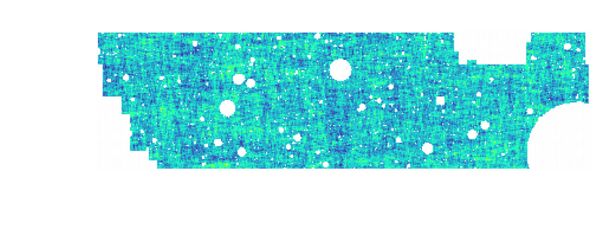
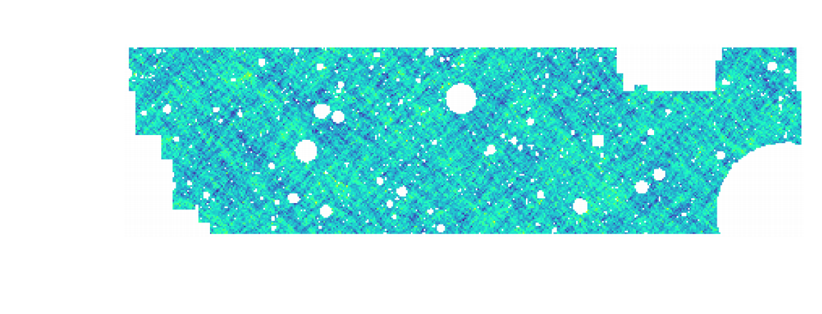
- Convergence map at z=1.0, based on a 3D simulation of $128^3$ particles for side. The 2D lensing map has an angular extent of $5^{\circ}.$
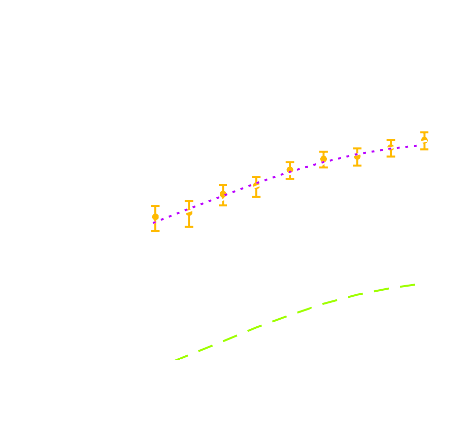
- Angular Power Spectrum $C_\ell$


Proof of Concept: Peak counts


Proof of Concept: $l_1$norm

- We take the sum of all wavelet coefficients of the original image $\kappa$ map in a given bin $i$ defined by two values, $B_i$ and $B_{i+1}$,
- Non-Gaussian information
- Information encoded in all pixels
- Avoids the problem of defining peaks and voids

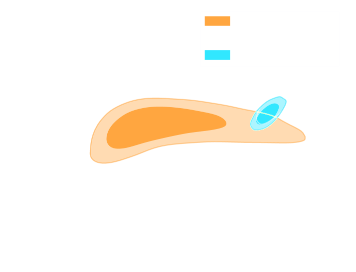
A first application: Fisher forecasts
We are testing the simulations to reproduce a LSST Y1-like setting
(Preliminary results, presented on behalf of LSST DESC)
\[\begin{equation}
F_{\alpha, \beta} =\sum_{i,j} \frac{d\mu_i}{d\theta_{\alpha}}
C_{i,j}^{-1} \frac{d\mu_j}{d\theta_{\beta}}
\end{equation} \]
- Use Fisher matrix to estimate the information content extracted with a given statistic
- Derivative of summary statistics respect to the cosmological parameters.
e.g. the $\Omega_c$, $\sigma_8$ - Fisher matrices are notoriously unstable
$\Longrightarrow$ they rely on evaluating gradients by finite differences. - They do not scale well to large number of parameters.
A first application: Fisher forecasts

A first application: Fisher forecasts

Fisher constraints from the full peak count statistics
Conclusion
Conclusion
What can be gained by simulating the Universe in a fast and differentiable way?
- Investigate the constraining power of various map-based higher order weak lensing statistics and control the systematics
- Differentiable physical models for fast inference ( made efficient by very fast lensing lightcone and having access to gradient)
- Even analytic cosmological computations can benefit from differentiability.
Thank you !