Forecasting the power of higher order weak lensing statistics with automatically differentiable simulations
Denise Lanzieri


the $\Lambda$CDM view of the Universe


Weak Gravitational lensing
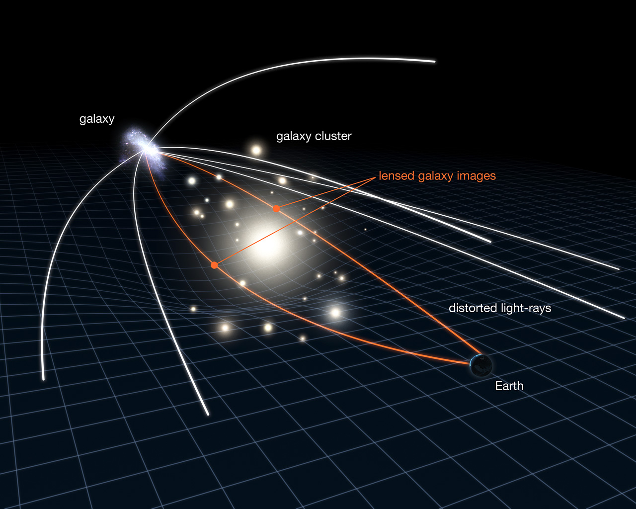
Weak Gravitational Lensing

Weak Gravitational Lensing

Weak lensing power spectrum
The lensing convergence is related to the projection of the 3D cosmological mass density perturbations along the line-of-sight.
\begin{equation} \kappa(\boldsymbol{\theta})= \frac{3H_0^2 \Omega_m}{2c^2} \int_0^{\inf} d\chi \frac{\chi}{a(\chi)} W(\chi,\chi_s) \delta(\chi \boldsymbol{\theta},\chi). \end{equation}
The cosmological information contained in cosmic shear data on large linear scales is well captured by two-point statistics in the form of the lensing power spectrum $C_{\ell}$ (or the shear two-point correlation functions):
\begin{equation} \left \langle \tilde{\kappa}(\ell)\tilde{\kappa}^{*}(\ell') \right \rangle =(2 \pi)^2\delta_{D}(\ell-\ell')P_{k}(\ell) \end{equation}
the Rubin Observatory Legacy Survey of Space and Time
- 1000 images each night, 15 TB/night for 10 years
- 18,000 square degrees, observed once every few days
- Tens of billions of objects, each one observed $\sim1000$ times
$\Longrightarrow$ Incredible potential for discovery, along with unprecedented challenges.
The challenges of modern surveys
$\Longrightarrow$ Modern surveys will provide large volumes of high quality data
A Blessing
- Unprecedented statistical power
- Great potential for new discoveries
A Curse
- Existing methods are reaching their limits at every step of the science analysis
- Control of systematic uncertainties becomes paramount
LSST forecast on dark energy parameters
![]()
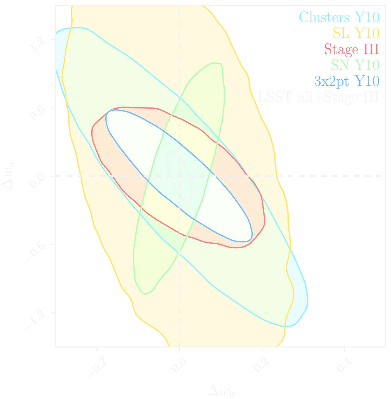
$\Longrightarrow$ Dire need for novel analysis techniques to fully realize the potential of modern surveys.
Traditional cosmological inference
How do we make the most of the available data?
HSC cosmic shear power spectrum
HSC Y1 constraints on $(S_8, \Omega_m)$
(Hikage,..., Lanusse, et al. 2018)
- Data reduction
- Compute summary statistics based on 2pt functions,
e.g. the power spectrum - Run an MCMC to recover a posterior on model parameters, using an analytic likelihood $$ p(\theta | x ) \propto \underbrace{p(x | \theta)}_{\mathrm{likelihood}} \ \underbrace{p(\theta)}_{\mathrm{prior}}$$
Main limitation: The lensing convergence field is inherently and significantly non-Gaussian
The two-point statistics do not fully capture the non-Gaussian information encoded in the peaks of the matter distribution
$\Longrightarrow$ We are dismissing most of the information!
2 Point Statistics: A Suboptimal Measure


How to maximize the information gain?

(Ajani, et al. 2020)
- Approaches based on measuring high-order correlations to access the non-Gaussian information
e.g. the Peaks count - Simulation-based approaches
Main limitation: Gradient-based
Numerical Differentiation
\[\begin{equation}
\left.\frac{df(x)}{dx}\right|_{x_1} \approx \frac{f(x_1+h)-f(x_1)}{h}
\end{equation} \]

-
Flaws :
- It’s numerically very unstable
- It’s very expensive in term of simulation time
- Computes an approximation
Different approach :
Automatic Differentiation
Automatic Differentiation
Automatic Differentiation and Gradients in TensorFlow
- Automatic differentiation allows you to compute analytic derivatives of arbitraty expressions:
If I form the expression $y = a * x + b$, it is separated in fundamental ops: $$ y = u + b \qquad u = a * x $$ then gradients can be obtained by the chain rule: $$\frac{\partial y}{\partial x} = \frac{\partial y}{\partial u} \frac{ \partial u}{\partial x} = 1 \times a = a$$ - To differentiate automatically, TensorFlow remember what operations happen in what order during the forward pass and traverses this list of operations in reverse order to compute gradients.
-
Advantages :
- Derivative as functions
- No numerical approximation
- High speed

Cosmological N-Body Simulations
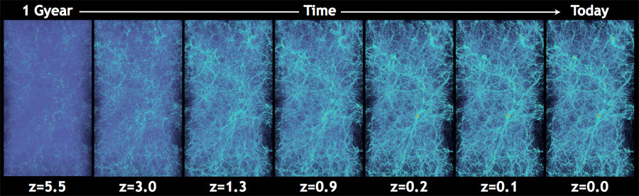
How do we simulate the Universe in a fast and differentiable way?
The Particle-Mesh scheme for N-body simulations
The idea: approximate gravitational forces by estimating densities on a grid.- The numerical scheme:
- Estimate the density of particles on a mesh
$\Longrightarrow$ compute gravitational forces by FFT - Interpolate forces at particle positions
- Update particle velocity and positions, and iterate
- Estimate the density of particles on a mesh
- Fast and simple, at the cost of approximating short range interactions.
$\Longrightarrow$ Only a series of FFTs and interpolations.
Introducing FlowPM: Particle-Mesh Simulations in TensorFlow

											import tensorflow as tf
											import flowpm
											# Defines integration steps
											stages = np.linspace(0.1, 1.0, 10, endpoint=True)

											initial_conds = flowpm.linear_field(32,        # size of the cube
											100,       # Physical size
											ipklin,    # Initial powerspectrum
											batch_size=16)

											# Sample particles and displace them by LPT
											state = flowpm.lpt_init(initial_conds, a0=0.1)

											# Evolve particles down to z=0
											final_state = flowpm.nbody(state, stages, 32)

											# Retrieve final density field
											final_field = flowpm.cic_paint(tf.zeros_like(initial_conditions),
											final_state[0])

											with tf.Session() as sess:
											sim = sess.run(final_field)
- Seamless interfacing with deep learning components
Potential Gradient Descent (PGD)
-
Flow N-body PM simulation:
- Fast (limited number of time steps while enforcing the correct linear growth)
- Cannot give accurate halo matter profiles or matter power spectrum
The PGD idea : mimics the physics that is missing
$\Longrightarrow$ Halo virialization

(Biwei Dai et al. 2018)
Potential Gradient Descent (PGD)
- Additional displacements to sharpen the halos
- The direction of the displacements points towards the halo center (local potential minimum).
- The gravitational force: \begin{equation} \mathbf{F}=-\nabla\Phi \end{equation}
- The PGD correction displacement: \begin{equation} \mathbf{S}=-\alpha\nabla \hat{O}_{h}\hat{O}_{l}\Phi \end{equation} High pass filter prevents the large scale growth, low pass filter reduces the numerical effect
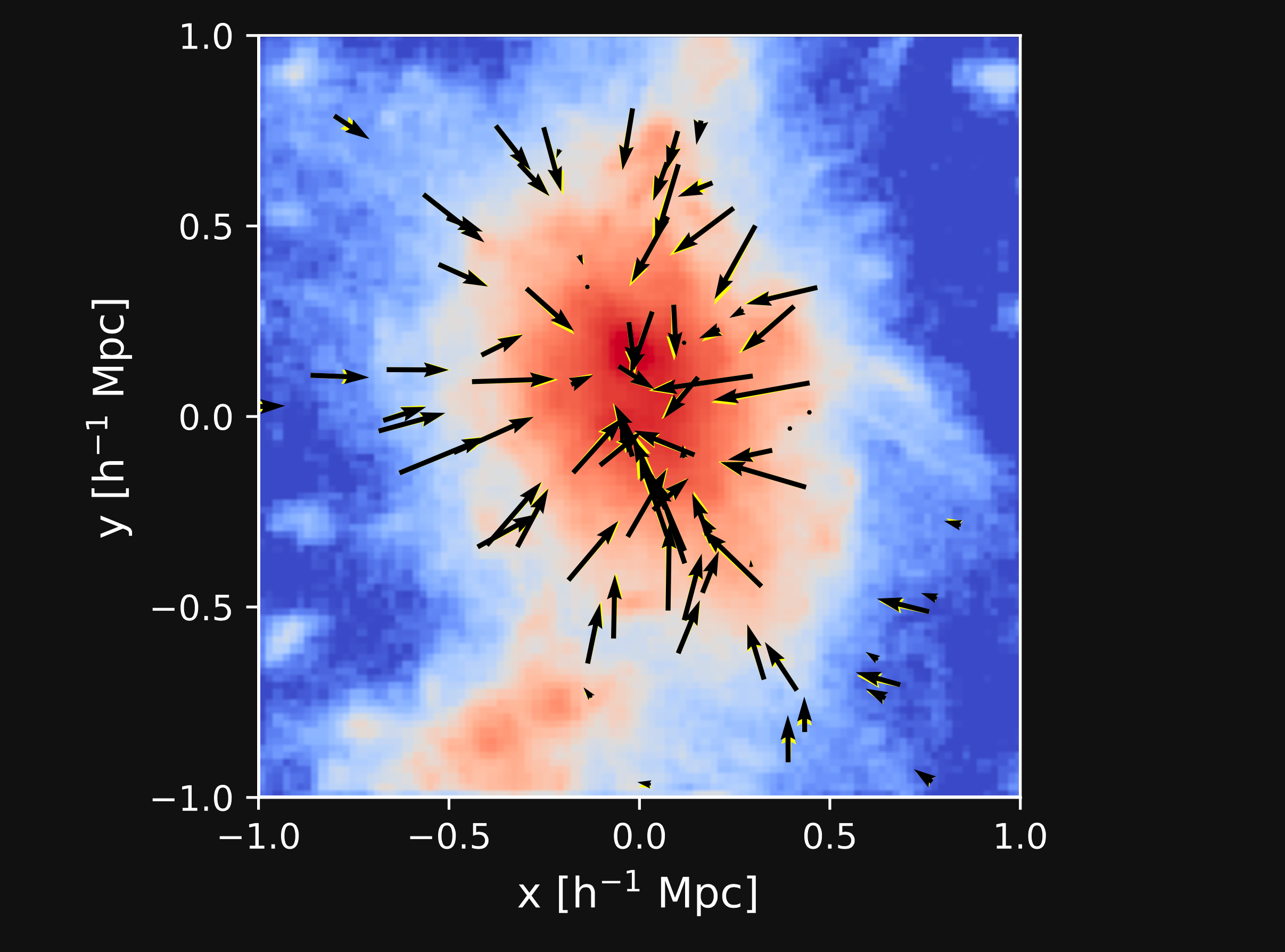
(Biwei Dai et al. 2018)
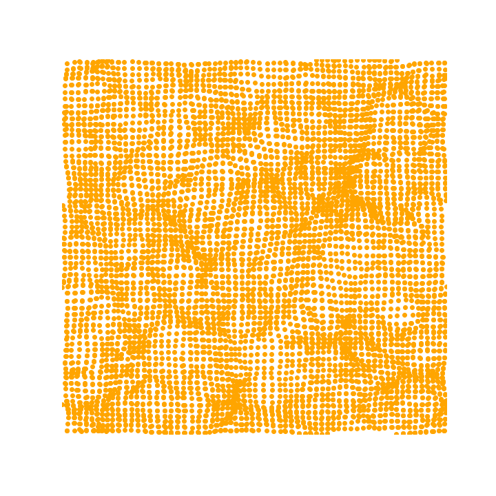
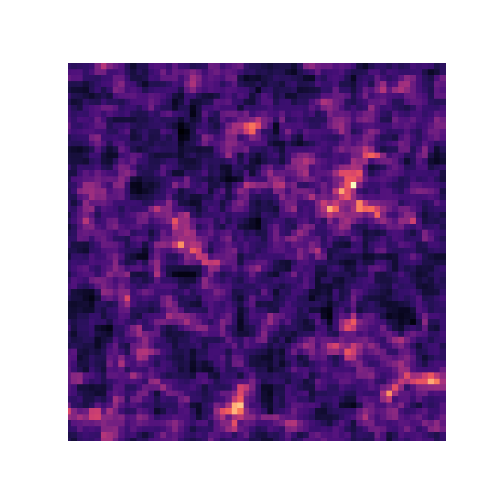
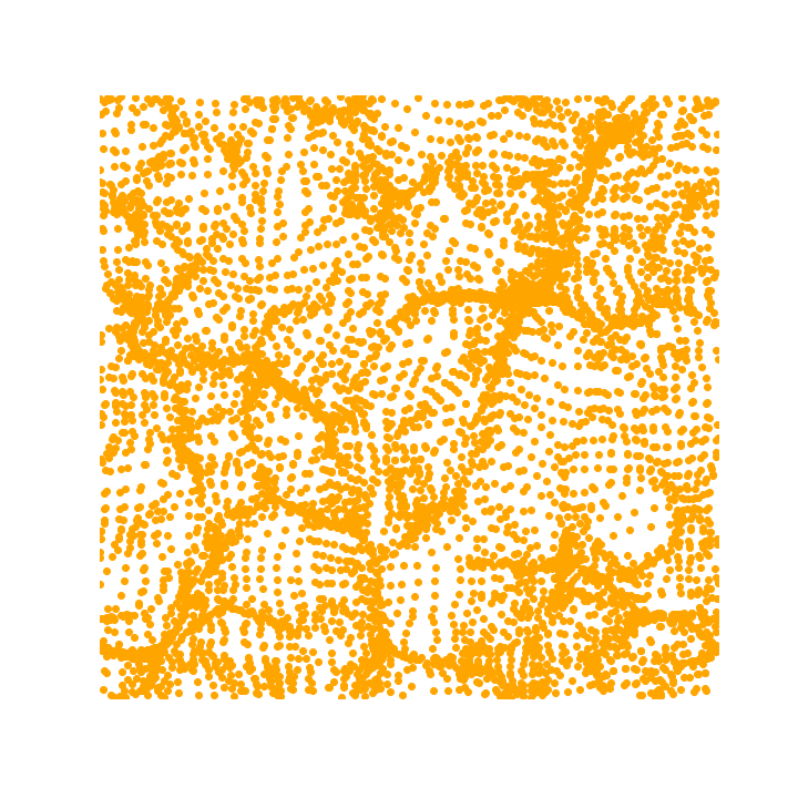
Potential Gradient Descent (PGD)
Result on a density map (z=0.03) with PGD turned off (left) and turned on (right):

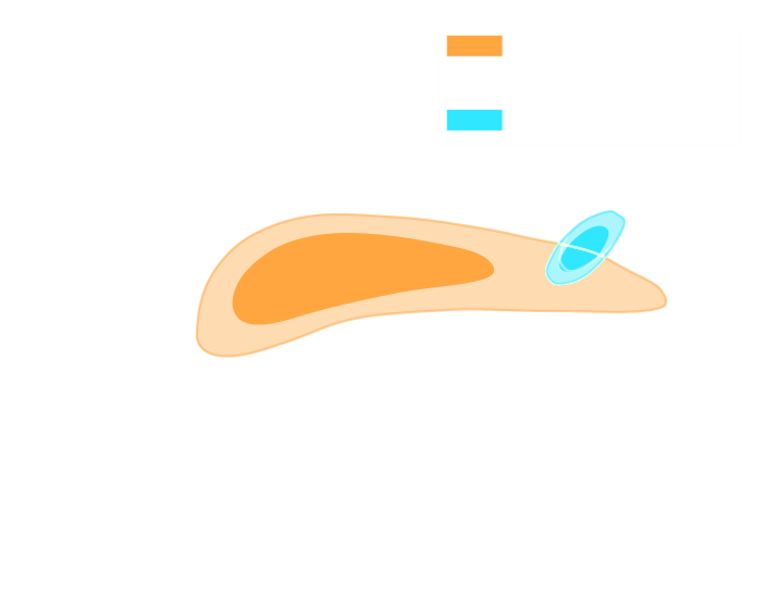
Mocking the weak lensing universe: The Born Approximation
- Numerical simulation of WL features rely on ray-tracing through the output of N-body simulations
- Knowledge of the Gravitational potential and accurate solvers for light ray trajectories is computationally expensive
- Born approximation , only requiring knowledge of the density field, can be implemented more efficiently and at a lower computational cost
\[\begin{equation} \kappa_{born}(\boldsymbol{\theta},\chi_s)= \frac{3H_0^2 \Omega_m}{2c^2} \int_0^{\chi_s} d\chi \frac{\chi}{a(\chi)} W(\chi,\chi_s) \delta(\chi \boldsymbol{\theta},\chi). \end{equation} \]
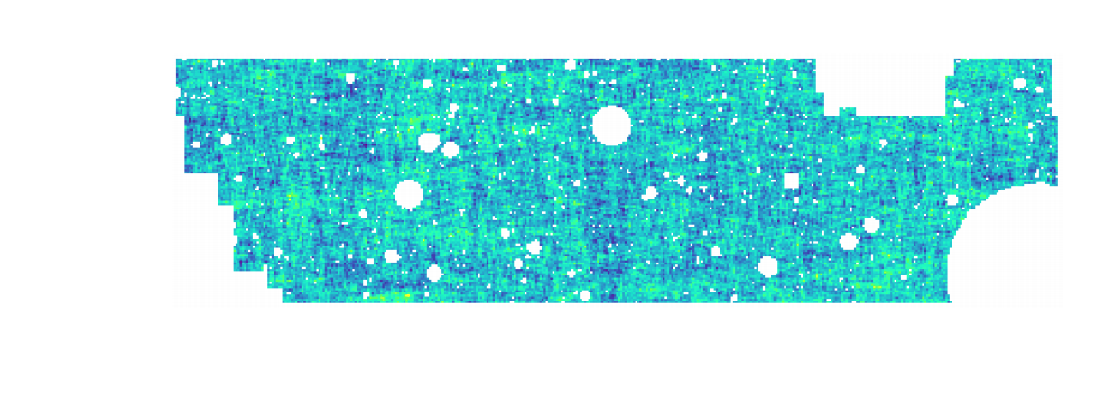
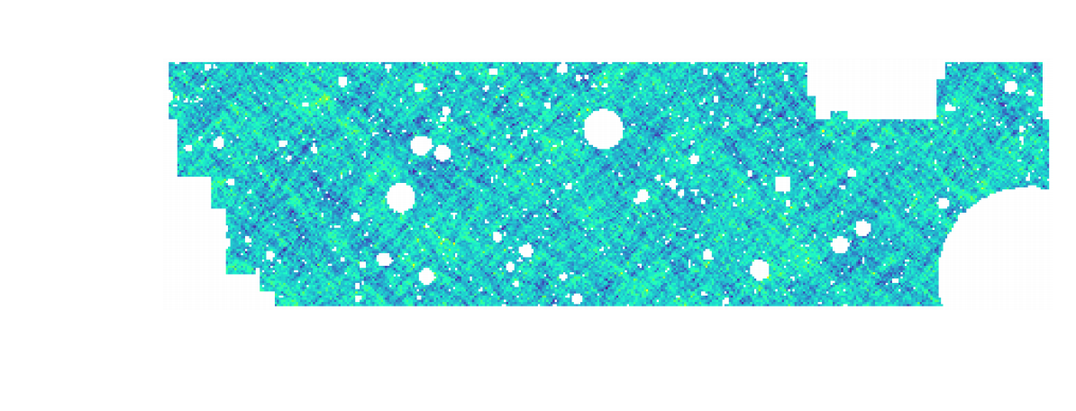
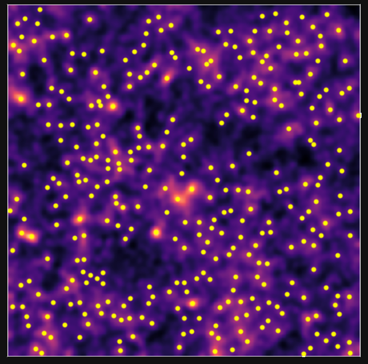
Proof of Concept
- Convergence map at z=1.0, based on a 3D simulation of $128^3$ particles for side. The 2D lensing map has an angular extent of $5^{\circ}.$
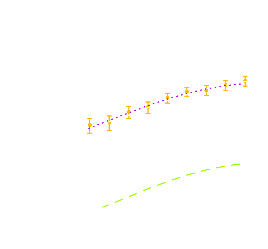
- Angular Power Spectrum $C_\ell$
We are testing the simulations to reproduce a DESC Y1-like setting


Proof of Concept: Peak counts

Proof of Concept: $l_1$norm

- We take the sum of all wavelet coefficients of the original image $\kappa$ map in a given bin $i$ defined by two values, $B_i$ and $B_{i+1}$,
- Non-Gaussian information
- Information encoded in all pixels
- Avoids the problem of defining peaks and voids
A first application: Fisher forecasts
\[\begin{equation}
F_{\alpha, \beta} =\sum_{i,j} \frac{d\mu_i}{d\theta_{\alpha}}
C_{i,j}^{-1} \frac{d\mu_j}{d\theta_{\beta}}
\end{equation} \]
- Derivative of summary statistics respect to the cosmological parameters.
e.g. the $\Omega_c$, $\sigma_8$ - The main reason for using Fisher matrices is that full MCMCs are extremely slow, and get slower with dimensionality.
- Fisher matrices are notoriously unstable
$\Longrightarrow$ they rely on evaluating gradients by finite differences. - They do not scale well to large number of parameters.
A first application: Fisher forecasts

A first application: Fisher forecasts

Intrinsic alignments of galaxies
 $$ \underbrace{\epsilon}_{\tiny \mbox{observed ellipticity}} = \underbrace{\epsilon_i}_{\tiny \mbox{intrinsic ellipticity}} + \underbrace{\gamma}_{\tiny \mbox{lensing}}$$
assuming $< \epsilon_i \epsilon_i^\prime > = 0$

Harnois-Déraps et al. (2021)
Infusion of intrinsic alignments


Intrinsic alignments: Validation and next steps
- Validate our infusion model by comparing two-point statistics against predictions from the IA model and prove to recover good match
- Measure the impact of the IA on three different statistics: angular power spectrum, peaks, $l_1$norm

Harnois-Déraps et al. (2021)
Summary
- We implement fast and accurate FlowPM N-body simulations based on the TensorFlow framework to model
the Large-Scale Structure in a fast and differentiable way.
- We simulate lensing lightcones implementing gravitational lensing ray-tracing in this framework
- We take derivatives of the summary statistic resulting on the gravitational lensing maps with respect to cosmological parameters (or any systematics included in the simulations)
- We use these derivatives to measure the Fisher information content of lensing summary statistics on cosmological parameters
Conclusion
Conclusion
What can be gained by simulating the Universe in a fast and differentiable way?
- Differentiable physical models for fast inference ( made efficient by very fast lensing lightcone and having access to gradient)
- Even analytic cosmological computations can benefit from differentiability.
- Investigate the constraining power of various map-based higher order weak lensing statistics and control the systematics
Thank you !